Squid's Blog

If you look long enough into the autoencoder, it looks back at you.

The Autoencoder is a fun deep learning model to look into. Its goal is simple: given an input image, we would like to have the same output image.

It’s sort of an identity function for deep learning models, but it is composed of two parts: an encoder and decoder, with the encoder translating the images to a latent space representation and the encoder translating that back to a regular images that we can view.

We are going to make a simple autoencoder with Clojure MXNet for handwritten digits using the MNIST dataset.

The Dataset

We first load up the training data into an iterator that will allow us to cycle through all the images.

1
2
3
4
5
6

(def train-data (mx-io/mnist-iter {:image (str data-dir "train-images-idx3-ubyte")
                                   :label (str data-dir "train-labels-idx1-ubyte")
                                   :input-shape [784]
                                   :flat true
                                   :batch-size batch-size
                                   :shuffle true}))

Notice there the the input shape is 784. We are purposely flattening out our 28x28 image of a number to just be a one dimensional flat array. The reason is so that we can use a simpler model for the autoencoder.

We also load up the corresponding test data.

1
2
3
4
5
6

(def test-data (mx-io/mnist-iter {:image (str data-dir "t10k-images-idx3-ubyte")
                                  :label (str data-dir "t10k-labels-idx1-ubyte")
                                  :input-shape [784]
                                  :batch-size batch-size
                                  :flat true
                                  :shuffle true}))

When we are working with deep learning models we keep the training and the test data separate. When we train the model, we won’t use the test data. That way we can evaluate it later on the unseen test data.

The Model

Now we need to define the layers of the model. We know we are going to have an input and an output. The input will be the array that represents the image of the digit and the output will also be an array which is reconstruction of that image.

1
2
3
4
5
6
7
8
9
10
11
12
13
14
15
16
17
18
19
20
21
22
23
24
25
26

(def input (sym/variable "input"))
(def output (sym/variable "input_"))

(defn get-symbol []
  (as-> input data
    ;; encode
    (sym/fully-connected "encode1" {:data data :num-hidden 100})
    (sym/activation "sigmoid1" {:data data :act-type "sigmoid"})

    ;; encode
    (sym/fully-connected "encode2" {:data data :num-hidden 50})
    (sym/activation "sigmoid2" {:data data :act-type "sigmoid"})

    ;; decode
    (sym/fully-connected "decode1" {:data data :num-hidden 50})
    (sym/activation "sigmoid3" {:data data :act-type "sigmoid"})

    ;; decode
    (sym/fully-connected "decode2" {:data data :num-hidden 100})
    (sym/activation "sigmoid4" {:data data :act-type "sigmoid"})

    ;;output
    (sym/fully-connected "result" {:data data :num-hidden 784})
    (sym/activation "sigmoid5" {:data data :act-type "sigmoid"})

    (sym/linear-regression-output {:data data :label output})))

From the model above we can see the input (image) being passed through simple layers of encoder to its latent representation, and then boosted back up from the decoder back into an output (image). It goes through the pleasingly symmetric transformation of:

784 (image) -> 100 -> 50 -> 50 -> 100 -> 784 (output)

We can now construct the full model with the module api from clojure-mxnet.

1
2
3
4
5
6
7

(def data-desc (first (mx-io/provide-data-desc train-data)))

(def model (-> (m/module (get-symbol) {:data-names ["input"] :label-names ["input_"]})
               (m/bind {:data-shapes [(assoc data-desc :name "input")]
                        :label-shapes [(assoc data-desc :name "input_")]})
               (m/init-params {:initializer  (initializer/uniform 1)})
               (m/init-optimizer {:optimizer (optimizer/adam {:learning-rage 0.001})})))

Notice that when we are binding the data-shapes and label-shapes we are using only the data from our handwritten digit dataset, (the images), and not the labels. This will ensure that as it trains it will seek to recreate the input image for the output image.

Before Training

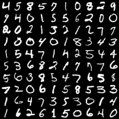
Before we start our training, let’s get a baseline of what the original images look like and what the output of the untrained model is.

To look at the original images we can take the first training batch of 100 images and visualize them. Since we are initially using the flattened [784] image representation. We need to reshape it to the 28x28 image that we can recognize.

1
2
3
4

(def my-batch (mx-io/next train-data))
(def images (mx-io/batch-data my-batch))
(ndarray/shape (ndarray/reshape (first images) [100 1 28 28]))
(viz/im-sav {:title "originals" :output-path "results/" :x (ndarray/reshape (first images) [100 1 28 28])})

We can also do the same visualization with the test batch of data images by putting them into the predict-batch and using our model.

1
2
3
4
5

;;; before training
 (def my-test-batch (mx-io/next test-data))
 (def test-images (mx-io/batch-data my-test-batch))
 (def preds (m/predict-batch model {:data test-images} ))
 (viz/im-sav {:title "before-training-preds" :output-path "results/" :x (ndarray/reshape (first preds) [100 1 28 28])})

They are not anything close to recognizable as numbers.

Training

The next step is to train the model on the data. We set up a training function to step through all the batches of data.

1
2
3
4
5
6
7
8
9
10
11
12
13
14

(def my-metric (eval-metric/mse))

(defn train [num-epochs]
  (doseq [epoch-num (range 0 num-epochs)]
    (println "starting epoch " epoch-num)
    (mx-io/do-batches
     train-data
     (fn [batch]
       (-> model
           (m/forward {:data (mx-io/batch-data batch) :label (mx-io/batch-data batch)})
           (m/update-metric my-metric (mx-io/batch-data batch))
           (m/backward)
           (m/update))))
    (println "result for epoch " epoch-num " is " (eval-metric/get-and-reset my-metric))))

For each batch of 100 images it is doing the following:

• Run the forward pass of the model with both the data and label being the image
• Update the accuracy of the model with the mse (mean squared error metric)
• Do the backward computation
• Update the model according to the optimizer and the forward/backward computation.

Let’s train it for 3 epochs.

1
2
3
4
5
6

starting epoch  0
result for epoch  0  is  [mse 0.06460866]
starting epoch  1
result for epoch  1  is  [mse 0.033874355]
starting epoch  2
result for epoch  2  is  [mse 0.027255038]

After training

We can check the test images again and see if they look better.

1
2
3
4
5

;;; after training
(def my-test-batch (mx-io/next test-data))
(def test-images (mx-io/batch-data my-test-batch))
(def preds (m/predict-batch model {:data test-images} ))
(viz/im-sav {:title "after-training-preds" :output-path "results/" :x (ndarray/reshape (first preds) [100 1 28 28])})

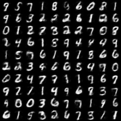
Much improved! They definitely look like numbers.

Wrap up

We’ve made a simple autoencoder that can take images of digits and compress them down to a latent space representation the can later be decoded into the same image.

If you want to check out the full code for this example, you can find it here.

Stay tuned. We’ll take this example and build on it in future posts.

Spring is bringing some beautiful new things to the Clojure MXNet. Here are some highlights for the month of April.

Shipped

We’ve merged 10 PRs over the last month. Many of them focus on core improvements to documentation and usability which is very important.

The MXNet project is also preparing a new release 1.4.1, so keep on the lookout for that to hit in the near future.

Clojure MXNet Made Simple Article Series

Arthur Caillau added another post to his fantastic series - MXNet made simple: Pretrained Models for image classification - Inception and VGG

Cool Stuff in Development

New APIs

Great progress was made on the new version of the API for the Clojure NDArray and Symbol APIs by Kedar Bellare. We now have an experimental new version of the apis that are generated more directly from the C code so that we can have more control over the output.

For example the new version of the generated api for NDArray looks like:

1
2
3
4
5
6
7
8
9
10
11
12
13
14
15
16
17
18
19
20
21
22
23

(defn
 activation
 "Applies an activation function element-wise to the input.
  
  The following activation functions are supported:
  
  - `relu`: Rectified Linear Unit, :math:`y = max(x, 0)`
  - `sigmoid`: :math:`y = \\frac{1}{1 + exp(-x)}`
  - `tanh`: Hyperbolic tangent, :math:`y = \\frac{exp(x) - exp(-x)}{exp(x) + exp(-x)}`
  - `softrelu`: Soft ReLU, or SoftPlus, :math:`y = log(1 + exp(x))`
  - `softsign`: :math:`y = \\frac{x}{1 + abs(x)}`
  
  
  
  Defined in src/operator/nn/activation.cc:L167
  
  `data`: The input array.
  `act-type`: Activation function to be applied.
  `out`: Output array. (optional)"
 ([data act-type] (activation {:data data, :act-type act-type}))
 ([{:keys [data act-type out], :or {out nil}, :as opts}]
  (util/coerce-return
   (NDArrayAPI/Activation data act-type (util/->option out)))))

as opposed to:

1
2
3
4
5
6
7
8

(defn
 activation
 ([& nd-array-and-params]
  (util/coerce-return
   (NDArray/Activation
    (util/coerce-param
     nd-array-and-params
     #{"scala.collection.Seq"})))))

So much nicer!!!

BERT (State of the Art for NLP)

We also have some really exciting examples for BERT in a PR that will be merged soon. If you are not familiar with BERT, this blog post is a good overview. Basically, it’s the state of the art in NLP right now. With the help of exported models from GluonNLP, we can do both inference and fine tuning of BERT models in MXNet with Clojure! This is an excellent example of cross fertilization across the GluonNLP, Scala, and Clojure MXNet projects.

There are two examples.

1) BERT question and answer inference based off of a fine tuned model of the SQuAD Dataset in GluonNLP which is then exported. It allows one to actually do some natural language question and answering like:

1
2
3
4
5
6
7

Question Answer Data
{:input-answer
 "Rich Hickey is the creator of the Clojure language. Before Clojure, he developed dotLisp, a similar project based on the .NET platform, and three earlier attempts to provide interoperability between Lisp and Java: a Java foreign language interface for Common Lisp, A Foreign Object Interface for Lisp, and a Lisp-friendly interface to Java Servlets.",
 :input-question "Who created Clojure?",
 :ground-truth-answers ["rich" "hickey"]}

  Predicted Answer:  [rich hickey]

2) The second example is using the exported BERT base model and then fine tuning it in Clojure to do a task with sentence pair classification to see if two sentences are equivalent or not.

The nice thing about this is that we were able to convert the existing tutorial in GluonNLP over to a Clojure Jupyter notebook with the lein-jupyter plugin. I didn’t realize that there is a nifty save-as command in Jupyter that can generate a markdown file, which makes for very handy documentation. Take a peek at the tutorial here. It might make its way into a blog post on its own in the next week or two.

Upcoming Events

• I’ll be speaking about Clojure MXNet at the next Scicloj Event on May 15th at 10PM UTC. Please join us and get involved in making Clojure a great place for Data Science.

• I’m also really excited to attend ICLR in a couple weeks. It is a huge conference that I’m sure will melt my mind with the latest research in Deep Learning. If anyone else is planning to attend, please say hi :)

Get Involved

As always, we welcome involvement in the true Apache tradition. If you have questions or want to say hi, head on over the the closest #mxnet room on your preferred server. We are on Clojurian’s slack and Zulip

Cat Picture of the Month

To close out, let’s take a lesson from my cats and don’t forget the importance of naps.

Have a great rest of April!

I’m starting a monthly update for Clojure MXNet. The goal is to share the progress and exciting things that are happening in the project and our community.

Here’s some highlights for the month of March.

Shipped

Under the shipped heading, the 1.4.0 release of MXNet has been released, along with the Clojure MXNet Jars. There have been improvements to the JVM memory management and an Image API addition. You can see the full list of changes here

Clojure MXNet Made Simple Article Series

Arthur Caillau authored a really nice series of blog posts to help get people started with Clojure MXNet.

• Getting started with Clojure and MXNet on AWS
• MXNet made simple: Clojure NDArray API
• MXNet made simple: Clojure Symbol API
• MXNet made simple: Clojure Module API
• MXNet made simple: Clojure Symbol Visualization API
• MXNet made simple: Image Manipulation with OpenCV and MXNet

Lein Template & Docker file

Nicolas Modrzyk created a Leiningen template that allows you to easily get a MXNet project started - with a notebook too! It’s a great way to take Clojure MXNet for a spin

1
2
3
4
5
6
7
8
9
10
11
12
13

# create project
lein new clj-mxnet hello

# run included sample
lein run

# start notebook engine
lein notebook

# open notebook
http://0.0.0.0:10000/worksheet.html?filename=notes/practice.clj
# open empty notebook with all namespaces
http://0.0.0.0:10000/worksheet.html?filename=notes/empty.clj

There also is a docker file as well

1
2
3
4
5
6
7
8

docker run -it -p 10000:10000 hellonico/mxnet

After starting the container, you can open the same notebooks as above:

# open notebook
http://0.0.0.0:10000/worksheet.html?filename=notes/practice.clj
# open empty notebook with all namespaces
http://0.0.0.0:10000/worksheet.html?filename=notes/empty.clj

Cool Stuff in Development

There are a few really interesting things cooking for the future.

One is a PR for memory fixes from the Scala team that is getting really close to merging. This will be a solution to some the the memory problems that were encountered by early adopters of the Module API.

Another, is the new version of the API for the Clojure NDArray and Symbol APIs that is being spearheaded by Kedar Bellare

Finally, work is being started to create a Gluon API for the Clojure package which is quite exciting.

Get Involved

As always, we welcome involvement in the true Apache tradition. If you have questions or want to say hi, head on over the the closest #mxnet room on your preferred server. We are on Clojurian’s slack and Zulip.

Cat Picture of the Month

There is no better way to close out an update than a cat picture, so here is a picture of my family cat watching birds at the window.

Have a great rest of March!

Object detection just landed in MXNet thanks to the work of contributors Kedar Bellare and Nicolas Modrzyk. Kedar ported over the infer package to Clojure, making inference and prediction much easier for users and Nicolas integrated in his Origami OpenCV library into the the examples to make the visualizations happen.

We’ll walk through the main steps to use the infer object detection which include creating the detector with a model and then loading the image and running the inference on it.

Creating the Detector

To create the detector you need to define a couple of things:

• How big is your image?
• What model are you going to be using for object detection?

In the code below, we are going to be giving it an color image of size 512 x 512.

1
2
3
4
5
6
7

(defn create-detector []
  (let [descriptors [{:name "data"
                      :shape [1 3 512 512]
                      :layout layout/NCHW
                      :dtype dtype/FLOAT32}]
        factory (infer/model-factory model-path-prefix descriptors)]
    (infer/create-object-detector factory)))

• The shape is going to be [1 3 512 512].
  • The 1 is for the batch size which in our case is a single image.
  • The 3 is for the channels in the image which for a RGB image is 3
  • The 512 is for the image height and width.
• The layout specifies that the shape given is in terms of NCHW which is batch size, channel size, height, and width.
• The dtype is the image data type which will be the standard FLOAT32
• The model-path-prefix points to the place where the trained model we are using for object detection lives.

The model we are going to use is the Single Shot Multiple Box Object Detector (SSD). You can download the model yourself using this script.

How to Load an Image and Run the Detector

Now that we have a model and a detector, we can load an image up and run the object detection.

To load the image use load-image which will load the image from the path.

1

(infer/load-image-from-file input-image)

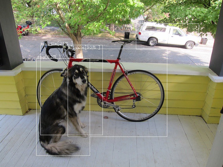
Then run the detection using infer/detect-objects which will give you the top five predictions by default.

1

(infer/detect-objects detector image)

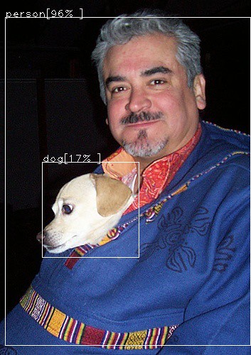
It will give an output something like this:

1
2
3
4
5
6
7
8
9
10
11
12
13
14

[[{:class "person",
   :prob 0.9657765,
   :x-min 0.021868259,
   :y-min 0.049295247,
   :x-max 0.9975169,
   :y-max 0.9734151}
  {:class "dog",
   :prob 0.17513266,
   :x-min 0.16772352,
   :y-min 0.45792937,
   :x-max 0.55409217,
   :y-max 0.72507095}
   ...
]]

which you can then use to draw bounding boxes on the image.

Try Running the Example

One of the best ways to explore using it is with the object detection example in the MXNet repo. It will be coming out officially in the 1.5.0 release, but you can get an early peek at it by building the project and running the example with the nightly snapshot.

You can do this by cloning the MXNet Repo and changing directory to contrib/clojure-package.

Next, edit the project.clj to look like this:

1
2
3
4
5
6
7
8
9
10
11
12
13
14
15
16
17
18
19
20
21
22
23
24
25
26
27
28
29
30
31
32

(defproject org.apache.mxnet.contrib.clojure/clojure-mxnet "1.5.0-SNAPSHOT"
  :description "Clojure package for MXNet"
  :url "https://github.com/apache/incubator-mxnet"
  :license {:name "Apache License"
            :url "http://www.apache.org/licenses/LICENSE-2.0"}
  :dependencies [[org.clojure/clojure "1.9.0"]
                 [t6/from-scala "0.3.0"]

                 ;; To use with nightly snapshot
                 ;[org.apache.mxnet/mxnet-full_2.11-osx-x86_64-cpu "<insert-snapshot-version>"]
                 ;[org.apache.mxnet/mxnet-full_2.11-linux-x86_64-cpu "<insert-snapshot-version>"]
                 ;[org.apache.mxnet/mxnet-full_2.11-linux-x86_64-gpu "<insert-snapshot-version"]

                 [org.apache.mxnet/mxnet-full_2.11-osx-x86_64-cpu "1.5.0-SNAPSHOT"]

                 ;;; CI
                 #_[org.apache.mxnet/mxnet-full_2.11 "INTERNAL"]

                 [org.clojure/tools.logging "0.4.0"]
                 [org.apache.logging.log4j/log4j-core "2.8.1"]
                 [org.apache.logging.log4j/log4j-api "2.8.1"]
                 [org.slf4j/slf4j-log4j12 "1.7.25" :exclusions [org.slf4j/slf4j-api]]]
  :pedantic? :skip
  :plugins [[lein-codox "0.10.3" :exclusions [org.clojure/clojure]]
            [lein-cloverage "1.0.10" :exclusions [org.clojure/clojure]]
            [lein-cljfmt "0.5.7"]]
  :codox {:namespaces [#"^org\.apache\.clojure-mxnet\.(?!gen).*"]}
  :aot [dev.generator]
  :repositories [["staging" {:url "https://repository.apache.org/content/repositories/staging"                  :snapshots true
                             :update :always}]
                 ["snapshots" {:url "https://repository.apache.org/content/repositories/snapshots"               :snapshots true
                              :update :always}]])

If you are running on linux, you should change the mxnet-full_2.11-osx-x86_64-cpu to mxnet-full_2.11-linux-x86_64-cpu.

Next, go ahead and do lein test to make sure that everything builds ok. If you run into any trouble please refer to README for any missing dependencies.

After that do a lein install to install the clojure-mxnet jar to your local maven. Now you are ready to cd examples/infer/object-detection to try it out. Refer to the README for more details.

If you run into any problems getting started, feel free to reach out in the Clojurian #mxnet slack room or open an issue at the MXNet project. We are a friendly group and happy to help out.

Thanks again to the community for the contributions to make this possible. It’s great seeing new things coming to life.

Happy Object Detecting!

It’s holiday time and that means parties and getting together with friends. Bringing a baked good or dessert to a gathering is a time honored tradition. But what if this year, you could take it to the next level? Everyone brings actual food. But with the help of Deep Learning, you can bring something completely different - you can bring the image of baked good! I’m not talking about just any old image that someone captured with a camera or created with a pen and paper. I’m talking about the computer itself creating. This image would be never before seen, totally unique, and crafted by the creative process of the machine.

That is exactly what we are going to do. We are going to create a flan

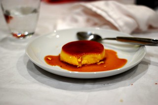
If you’ve never had a flan before, it’s a yummy dessert made of a baked custard with caramel sauce on it.

“Why a flan?”, you may ask. There are quite a few reasons:

• It’s tasty in real life.
• Flan rhymes with GAN, (unless you pronounce it “Gaaahn”).
• Why not?

Onto the recipe. How are we actually going to make this work? We need some ingredients:

• Clojure - the most advanced programming language to create generative desserts.
• Apache MXNet - a flexible and efficient deep learning library that has a Clojure package.
• 1000-5000 pictures of flans - for Deep Learning you need data!

Gather Flan Pictures

The first thing you want to do is gather your 1000 or more images with a scraper. The scraper will crawl google, bing, or instagram and download pictures of mostly flans to your computer. You may have to eyeball and remove any clearly wrong ones from your stash.

Next, you need to gather all these images in a directory and run a tool called im2rec.py on them to turn them into an image record iterator for use with MXNet. This will produce an optimized format that will allow our deep learning program to efficiently cycle through them.

Run:

python3 im2rec.py --resize 28 root flan

to produce a flan.rec file with images resized to 28x28 that we can use next.

Load Flan Pictures into MXNet

The next step is to import the image record iterator into the MXNet with the Clojure API. We can do this with the io namespace.

Add this to your require:

[org.apache.clojure-mxnet.io :as mx-io]

Now, we can load our images:

1
2
3

(def flan-iter (mx-io/image-record-iter {:path-imgrec "flan.rec"
                                         :data-shape [3 28 28]
                                         :batch-size batch-size}))

Now, that we have the images, we need to create our model. This is what is actually going to do the learning and creating of images.

Creating a GAN model.

GAN stands for Generative Adversarial Network. This is a incredibly cool deep learning technique that has two different models pitted against each, yet both learning and getting better at the same time. The two models are a generator and a discriminator. The generator model creates a new image from a random noise vector. The discriminator then tries to tell whether the image is a real image or a fake image. We need to create both of these models for our network.

First, the discriminator model. We are going to use the symbol namespace for the clojure package:

1
2
3
4
5
6
7
8
9
10
11
12

(defn discriminator []
  (as-> (sym/variable "data") data
    (sym/convolution "d1" {:data data
                           :kernel [4 4]
                           :pad [3 3]
                           :stride [2 2]
                           :num-filter ndf
                           :no-bias true})
    (sym/batch-norm "dbn1" {:data data :fix-gamma true :eps eps})
    (sym/leaky-re-lu "dact1" {:data data :act-type "leaky" :slope 0.2})

  ...

There is a variable for the data coming in, (which is the picture of the flan), it then flows through the other layers which consist of convolutions, normalization, and activation layers. The last three layers actually repeat another two times before ending in the output, which tells whether it thinks the image was a fake or not.

The generator model looks similar:

1
2
3
4
5
6
7
8
9
10
11
12
13

(defn generator []
  (as-> (sym/variable "rand") data
    (sym/deconvolution "g1" {:data data
                             :kernel [4 4]
                             :pad [0 0]
                             :stride [1 1]
                             :num-filter
                             (* 4 ndf) :no-bias true})
    (sym/batch-norm "gbn1" {:data data :fix-gamma true :eps eps})
    (sym/activation "gact1" {:data data :act-type "relu"})
  
  ...
  

There is a variable for the data coming in, but this time it is a random noise vector. Another interesting point that is is using a deconvolution layer instead of a convolution layer. The generator is basically the inverse of the discriminator. It starts with a random noise vector, but that is translated up through the layers until it is expanded to a image output.

Next, we iterate through all of our training images in our flan-iter with reduce-batches. Here is just an excerpt where we get a random noise vector and have the generator run the data through and produce the output image:

1
2
3
4
5
6
7
8

(mx-io/reduce-batches
       flan-iter
       (fn [n batch]
         (let [rbatch (mx-io/next rand-noise-iter)
               dbatch (mapv normalize-rgb-ndarray (mx-io/batch-data batch))
               out-g (-> mod-g
                         (m/forward rbatch)
                         (m/outputs))

The whole code is here for reference, but let’s skip forward and run it and see what happens.

FLANS!! Well, they could be flans if you squint a bit.

Now that we have them kinda working for a small image size 28x28, let’s biggerize it.

Turn on the Oven and Bake

Turning up the size to 128x128 requires some alterations in the layers’ parameters to make sure that it processes and generates the correct size, but other than that we are good to go.

Here comes the fun part, watching it train and learn:

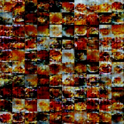
Epoch 0

In the beginning there was nothing but random noise.

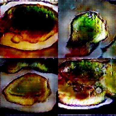
Epoch 10

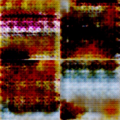
It’s beginning to learn colors! Red, yellow, brown seem to be important to flans.

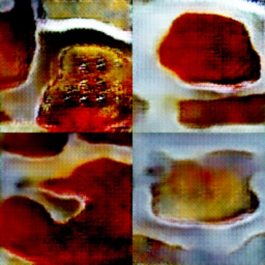
Epoch 23

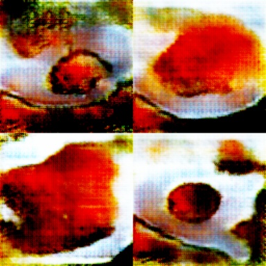
It’s learning shapes! It has learned that flans seem to be blob shaped.

Epoch 33

It is moving into its surreal phase. Salvidor Dali would be proud of these flans.

Epoch 45

Things take a weird turn. Does that flan have eyes?

Epoch 68

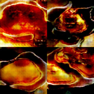
Even worse. Are those demonic flans? Should we even continue down this path?

Answer: Yes - the training must go on..

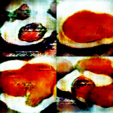
Epoch 161

Big moment here. It looks like something that could possibly be edible.

Epoch 170

Ick! Green Flans! No one is going to want that.

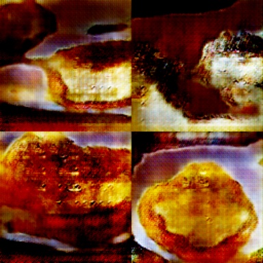
Epoch 195

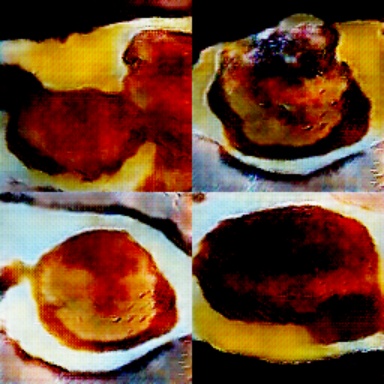
We’ve achieved maximum flan, (for the time being).

Explore

If you are interested in playing around with the pretrained model, you can check it out here with the pretrained function. It will load up the trained model and generate flans for you to explore and bring to your dinner parties.

Wrapping up, training GANs is a lot of fun. With MXNet, you can bring the fun with you to Clojure.

Want more, check out this Clojure Conj video - Can You GAN?.

This is an introduction to the high level Clojure API for deep learning library MXNet.

The module API provides an intermediate and high-level interface for performing computation with neural networks in MXNet.

To follow along with this documentation, you can use this namespace to with the needed requires:

1
2
3
4
5
6
7
8

(ns docs.module
  (:require [clojure.java.io :as io]
            [clojure.java.shell :refer [sh]]
            [org.apache.clojure-mxnet.eval-metric :as eval-metric]
            [org.apache.clojure-mxnet.io :as mx-io]
            [org.apache.clojure-mxnet.module :as m]
            [org.apache.clojure-mxnet.symbol :as sym]
            [org.apache.clojure-mxnet.ndarray :as ndarray]))

Prepare the Data

In this example, we are going to use the MNIST data set. If you have cloned the MXNet repo and cd contrib/clojure-package, we can run some helper scripts to download the data for us.

1
2
3
4

(def data-dir "data/")

(when-not (.exists (io/file (str data-dir "train-images-idx3-ubyte")))
  (sh "../../scripts/get_mnist_data.sh"))

MXNet provides function in the io namespace to load the MNIST datasets into training and test data iterators that we can use with our module.

1
2
3
4
5
6
7
8
9
10
11
12
13
14
15
16

(def train-data (mx-io/mnist-iter {:image (str data-dir "train-images-idx3-ubyte")
                                   :label (str data-dir "train-labels-idx1-ubyte")
                                   :label-name "softmax_label"
                                   :input-shape [784]
                                   :batch-size 10
                                   :shuffle true
                                   :flat true
                                   :silent false
                                   :seed 10}))

(def test-data (mx-io/mnist-iter {:image (str data-dir "t10k-images-idx3-ubyte")
                                  :label (str data-dir "t10k-labels-idx1-ubyte")
                                  :input-shape [784]
                                  :batch-size 10
                                  :flat true
                                  :silent false}))

Preparing a Module for Computation

To construct a module, we need to have a symbol as input. This symbol takes input data in the first layer and then has subsequent layers of fully connected and relu activation layers, ending up in a softmax layer for output.

1
2
3
4
5
6
7
8
9

(let [data (sym/variable "data")
      fc1 (sym/fully-connected "fc1" {:data data :num-hidden 128})
      act1 (sym/activation "relu1" {:data fc1 :act-type "relu"})
      fc2 (sym/fully-connected "fc2" {:data act1 :num-hidden 64})
      act2 (sym/activation "relu2" {:data fc2 :act-type "relu"})
      fc3 (sym/fully-connected "fc3" {:data act2 :num-hidden 10})
      out (sym/softmax-output "softmax" {:data fc3})]
  out)
  ;=>#object[org.apache.mxnet.Symbol 0x1f43a406 "org.apache.mxnet.Symbol@1f43a406"]

You can also write this with the as-> threading macro.

1
2
3
4
5
6
7
8

(def out (as-> (sym/variable "data") data
           (sym/fully-connected "fc1" {:data data :num-hidden 128})
           (sym/activation "relu1" {:data data :act-type "relu"})
           (sym/fully-connected "fc2" {:data data :num-hidden 64})
           (sym/activation "relu2" {:data data :act-type "relu"})
           (sym/fully-connected "fc3" {:data data :num-hidden 10})
           (sym/softmax-output "softmax" {:data data})))
;=> #'tutorial.module/out

By default, context is the CPU. If you need data parallelization, you can specify a GPU context or an array of GPU contexts like this (m/module out {:contexts [(context/gpu)]})

Before you can compute with a module, you need to call bind to allocate the device memory and init-params or set-params to initialize the parameters. If you simply want to fit a module, you don’t need to call bind and init-params explicitly, because the fit function automatically calls them if they are needed.

1
2
3
4
5

(let [mod (m/module out)]
  (-> mod
      (m/bind {:data-shapes (mx-io/provide-data train-data)
               :label-shapes (mx-io/provide-label train-data)})
      (m/init-params)))

Now you can compute with the module using functions like forward, backward, etc.

Training and Predicting

Modules provide high-level APIs for training, predicting, and evaluating. To fit a module, call the fit function with some data iterators:

1
2
3
4

(def mod (m/fit (m/module out) {:train-data train-data :eval-data test-data :num-epoch 1}))
;; Epoch  0  Train- [accuracy 0.12521666]
;; Epoch  0  Time cost- 8392
;; Epoch  0  Validation-  [accuracy 0.2227]

You can pass in batch-end callbacks using batch-end-callback and epoch-end callbacks using epoch-end-callback in the fit-params. You can also set parameters using functions like in the fit-params like optimizer and eval-metric. To learn more about the fit-params, see the fit-param function options. To predict with a module, call predict with a DataIter:

1
2
3
4

(def results (m/predict mod {:eval-data test-data}))
(first results) ;=>#object[org.apache.mxnet.NDArray 0x3540b6d3 "org.apache.mxnet.NDArray@a48686ec"]

(first (ndarray/->vec (first results))) ;=>0.08261358

The module collects and returns all of the prediction results. For more details about the format of the return values, see the documentation for the predict function.

When prediction results might be too large to fit in memory, use the predict-every-batch API.

1
2
3
4
5
6
7

(let [preds (m/predict-every-batch mod {:eval-data test-data})]
  (mx-io/reduce-batches test-data
                        (fn [i batch]
                          (println (str "pred is " (first (get preds i))))
                          (println (str "label is " (mx-io/batch-label batch)))
                          ;;; do something
                          (inc i))))

If you need to evaluate on a test set and don’t need the prediction output, call the score function with a data iterator and an eval metric:

1

(m/score mod {:eval-data test-data :eval-metric (eval-metric/accuracy)}) ;=>["accuracy" 0.2227]

This runs predictions on each batch in the provided data iterator and computes the evaluation score using the provided eval metric. The evaluation results are stored in metric so that you can query later.

Saving and Loading

To save the module parameters in each training epoch, use a checkpoint function:

1
2
3
4
5
6
7
8
9
10
11
12
13

(let [save-prefix "my-model"]
  (doseq [epoch-num (range 3)]
    (mx-io/do-batches train-data (fn [batch
                                          ;; do something
]))
    (m/save-checkpoint mod {:prefix save-prefix :epoch epoch-num :save-opt-states true})))

;; INFO  org.apache.mxnet.module.Module: Saved checkpoint to my-model-0000.params
;; INFO  org.apache.mxnet.module.Module: Saved optimizer state to my-model-0000.states
;; INFO  org.apache.mxnet.module.Module: Saved checkpoint to my-model-0001.params
;; INFO  org.apache.mxnet.module.Module: Saved optimizer state to my-model-0001.states
;; INFO  org.apache.mxnet.module.Module: Saved checkpoint to my-model-0002.params
;; INFO  org.apache.mxnet.module.Module: Saved optimizer state to my-model-0002.states

To load the saved module parameters, call the load-checkpoint function:

1
2
3

(def new-mod (m/load-checkpoint {:prefix "my-model" :epoch 1 :load-optimizer-states true}))

new-mod ;=> #object[org.apache.mxnet.module.Module 0x5304d0f4 "org.apache.mxnet.module.Module@5304d0f4"]

To initialize parameters, Bind the symbols to construct executors first with bind function. Then, initialize the parameters and auxiliary states by calling init-params function.

1
2
3

(-> new-mod
    (m/bind {:data-shapes (mx-io/provide-data train-data) :label-shapes (mx-io/provide-label train-data)})
    (m/init-params))

To get current parameters, use params

1
2
3
4
5
6
7
8
9
10
11
12
13
14
15
16
17
18

(let [[arg-params aux-params] (m/params new-mod)]
  {:arg-params arg-params
   :aux-params aux-params})

;; {:arg-params
;;  {"fc3_bias"
;;   #object[org.apache.mxnet.NDArray 0x39adc3b0 "org.apache.mxnet.NDArray@49caf426"],
;;   "fc2_weight"
;;   #object[org.apache.mxnet.NDArray 0x25baf623 "org.apache.mxnet.NDArray@a6c8f9ac"],
;;   "fc1_bias"
;;   #object[org.apache.mxnet.NDArray 0x6e089973 "org.apache.mxnet.NDArray@9f91d6eb"],
;;   "fc3_weight"
;;   #object[org.apache.mxnet.NDArray 0x756fd109 "org.apache.mxnet.NDArray@2dd0fe3c"],
;;   "fc2_bias"
;;   #object[org.apache.mxnet.NDArray 0x1dc69c8b "org.apache.mxnet.NDArray@d128f73d"],
;;   "fc1_weight"
;;   #object[org.apache.mxnet.NDArray 0x20abc769 "org.apache.mxnet.NDArray@b8e1c5e8"]},
;;  :aux-params {}}

To assign parameter and aux state values, use set-params function.

1
2

(m/set-params new-mod {:arg-params (m/arg-params new-mod) :aux-params (m/aux-params new-mod)})
;=> #object[org.apache.mxnet.module.Module 0x5304d0f4 "org.apache.mxnet.module.Module@5304d0f4"]

To resume training from a saved checkpoint, instead of calling set-params, directly call fit, passing the loaded parameters, so that fit knows to start from those parameters instead of initializing randomly

Create fit-params, and then use it to set begin-epoch so that fit knows to resume from a saved epoch.

1
2
3
4
5
6

;; reset the training data before calling fit or you will get an error
(mx-io/reset train-data)
(mx-io/reset test-data)

(m/fit new-mod {:train-data train-data :eval-data test-data :num-epoch 2
                :fit-params (-> (m/fit-params {:begin-epoch 1}))})

If you are interested in checking out MXNet and exploring on your own, check out the main page here with instructions on how to install and other information.

See other blog posts about MXNet

• Clojure MXNet - NDArray
• Clojure MXNet Joins Apache MXNet

I’m delighted to share the news that the Clojure package for MXNet has now joined the main Apache MXNet project. A big thank you to the efforts of everyone involved to make this possible. Having it as part of the main project is a great place for growth and collaboration that will benefit both MXNet and the Clojure community.

Invitation to Join and Contribute

The Clojure package has been brought in as a contrib clojure-package. It is still very new and will go through a period of feedback, stabilization, and improvement before it graduates out of contrib.

We welcome contributors and people getting involved to make it better.

Are you interested in Deep Learning and Clojure? Great - Join us!

There are a few ways to get involved.

• Check out the current state of the Clojure package some contribution needs here https://cwiki.apache.org/confluence/display/MXNET/Clojure+Package+Contribution+Needs
• Join the Clojurian Slack #mxnet channel
• Join the MXNet dev mailing list by sending an email to dev-subscribe@mxnet.apache.org..
• Join the MXNET Slack channel - You have to join the MXnet dev mailing list first, but after that says you would like to join the slack and someone will add you.
• Join the MXNet Discussion Forum

Want to Learn More?

There are lots of examples in the package to check out, but a good place to start are the tutorials here https://github.com/apache/incubator-mxnet/tree/master/contrib/clojure-package/examples/tutorial

There is a blog walkthough here as well - Clojure MXNet Module API

This is the beginning of a series of blog posts to get to know the Apache MXNet Deep Learning project and the new Clojure language binding clojure-package

MXNet is a first class, modern deep learning library that AWS has officially picked as its chosen library. It supports multiple languages on a first class basis and is incubating as an Apache project.

The motivation for creating a Clojure package is to be able to open the deep learning library to the Clojure ecosystem and build bridges for future development and innovation for the community. It provides all the needed tools including low level and high level apis, dynamic graphs, and things like GAN and natural language support.

So let’s get on with our introduction with one of the basic building blocks of MXNet, the NDArray.

Meet NDArray

The NDArray is the tensor data structure in MXNet. Let’s start of by creating one. First we need to require the ndarray namespace:

1
2

(ns tutorial.ndarray
  (:require [org.apache.clojure-mxnet.ndarray :as ndarray]))

Now let’s create an all zero array of dimension 100 x 50

1
2

(ndarray/zeros [100 50])
;=> #object[org.apache.mxnet.NDArray 0x3e396d0 "org.apache.mxnet.NDArray@aeea40b6"]

We can check the shape of this by using shape-vec

1
2

(ndarray/shape-vec (ndarray/zeros [100 50]))
;=> [100 50]

There is also a quick way to create an ndarray of ones with the ones function:

1

(ndarray/ones [256 32 128 1])

Ones and zeros are nice, but what an array with specific contents? There is an array function for that. Specific the contents of the array first and the shape second:

1
2

(def c (ndarray/array [1 2 3 4 5 6] [2 3]))
(ndarray/shape-vec c)  ;=> [2 3]

To convert it back to a vector format, we can use the ->vec function.

1
2

(ndarray/->vec c)
;=> [1.0 2.0 3.0 4.0 5.0 6.0]

Now that we know how to create NDArrays, we can get to do something interesting like operations on them.

Operations

There are all the standard arithmetic operations:

1
2
3
4

(def a (ndarray/ones [1 5]))
(def b (ndarray/ones [1 5]))
(-> (ndarray/+ a b) (ndarray/->vec))
;=>  [2.0 2.0 2.0 2.0 2.0]

Note that the original ndarrays are unchanged.

1
2

(ndarray/->vec a) ;=> [1.0 1.0 1.0 1.0 1.0]
(ndarray/->vec b) ;=> [1.0 1.0 1.0 1.0 1.0]

But, we can change that if we use the inplace operators:

1
2

(ndarray/+= a b)
(ndarray/->vec a) ;=>  [2.0 2.0 2.0 2.0 2.0]

There are many more operations, but just to give you a taste, we’ll take a look a the dot product operation:

1
2
3
4
5

(def arr1 (ndarray/array [1 2] [1 2]))
(def arr2 (ndarray/array [3 4] [2 1]))
(def res (ndarray/dot arr1 arr2))
(ndarray/shape-vec res) ;=> [1 1]
(ndarray/->vec res) ;=> [11.0]

If you are curious about the other operators available in NDArray API check out the MXNet project documentation page

Now that we have ndarrays and can do calculations on them, we might want to save and load them.

Saving and Loading

You can save ndarrays with a name as a map like:

1

(ndarray/save "filename" {"arr1" arr1 "arr2" arr2})

To load them, you just specify the filename and the map is returned.

1
2
3

(ndarray/load "filename")
;=> {"arr1" #object[org.apache.mxnet.NDArray 0x1b629ff4 "org.apache.mxnet.NDArray@63da08cb"]
;=>  "arr2" #object[org.apache.mxnet.NDArray 0x25d994e3 "org.apache.mxnet.NDArray@5bbaf2c3"]}

One more cool thing, we can even due our operations on the cpu or gpu.

Multi-Device Support

When creating an ndarray you can use a context argument to specify the device. To do this, we will need the help of the context namespace.

1

(require '[org.apache.clojure-mxnet.context :as context])

By default, the ndarray is created on the cpu context.

1
2
3

(def cpu-a (ndarray/zeros [100 200]))
(ndarray/context cpu-a)
;=> #object[ml.dmlc.mxnet.Context 0x3f376123 "cpu(0)"]

But we can specify the gpu instead, (if we have a gpu enabled build).

1

(def gpu-b (ndarray/zeros [100 200] {:ctx (context/gpu 0)}))

Note: Operations among different contexts are currently not allowed, but there is a copy-to function that can help copy the content from one device to another and then continue on with the computation.

Wrap up

I hope you’ve enjoyed the brief introduction to the MXNet library, there is much more to explore in future posts. If you are interested in giving it a try, there are native jars for OSX cpu and Linux cpu/gpu available and the code for the ndarray tutorial can be found here

Please remember that the library is in a experimential state, so if you encounter any problems or have any other feedback, please log an issue so bugs and rough edges can be fixed :).

I was 10 years into my career when I met her. I could count the number of other women programmers I had worked with on one hand and none of them had young children at home like me. She was not only incredibly experienced and competent, but also had a son in college. I was curious about her career path so I asked her one day at lunch why she was still programming and hadn’t become a manager instead.

She smiled at me kindly and replied, “I’ve worked very hard to stay exactly where I am”, and I was enlightened.

I wrote a blog post a while back about using a Clojure machine learning library called Cortex to do the Kaggle Cats and Dogs classification challenge.

I wanted to revisit it for a few reasons. The first one is that the Cortex library has progressed and improved considerably over the last year. It’s still not at version 1.0, but it my eyes, it’s really starting to shine. The second reason is that they recently published an example of using the RESNET50 model, (I’ll explain later on), to do fine-tuning or transfer learning. The third reason, is that there is a great new plugin for leiningen the supports using Jupyter notebooks with Clojure projects. These notebooks are a great way of doing walkthroughs and tutorials.

Putting all these things together, I felt like I was finally at a stage where I could somewhat replicate the first lesson in the Practical Deep Learning Course for Coders with Cats and Dogs - although this time all in Clojure!

Where to Start?

In the last blog post, we created our deep learning network and trained the data on scaled down images (like 50x50) from scratch. This time we are much smarter.

We are still of course going to have to get a hold of all the training data from Kaggle Cats vs Dogs Challenge. The big difference is this time, we are just going to have to train our model for 1 epoch. What’s more, the results will be way better than before.

How is this possible? We are going to use an already trained model, RESNET50. This model has already been painstakingly trained with a gigantic network that is 50 layers deep on the ImageNet challenge. That’s a challenge that has models try to classify a 1000 different categories. The theory is that the inner layers of the network have already learned about the features that make up cats and dogs, all we would need to do is peel off the final layer of the network and graft on a new layers that just learns the final classification for our 2 categories of cats and dogs. This is called transfer learning or retraining.

Plan of Action

• Get all the cats and dogs pictures in the right directory format for training
• Train the model with all but the last layer in the RESNET model. The last layer we are going to replace with our own layer that will finetune it to classify only cats and dogs
• Run the test data and come up with a spreadsheet of results to submit to Kaggle.

Getting all the data pictures in the right format

This is the generally the most time consuming step of most deep learning. I’ll spare you the gritty details but we want to get all the pictures from the train.zip into the format

1
2
3
4
5
6
7
8
9
10
11
12
13
14
15

-data
  -cats-dogs-training
      -cat
          1110.png
          ...
      -dog
          12416.png
          ...
  -cats-dogs-testing
      -cat
          11.png
          ...
      -dog
          12.png
          ...

The image sizes must also all be resized to match the input of the RESNET50. That means they all have to be 224x224.

Train the model

The cortex functions allow you to load the resnet50 model, remove the last layer, freeze all the other layers so that they will not be retrained, and add new layers.

I was surprised that I could actually train the model with all the images at 224x244 with the huge RESNET50 model. I built the uberjar and ran it which helped the performance.

lein uberjar

java -jar target/cats-dogs-cortex-redux.jar

Training one epoch took me approximately 6 minutes. Not bad, especially considering that’s all the training I really needed to do.

1
2

Loss for epoch 1: (current) 0.05875186542016347 (best) null
Saving network to trained-network.nippy

The key point is that it saved the fine tuned network to trained-network.nippy

Run the Kaggle test results and submit the results

You will need to do a bit more setup for this. First, you need to get the Kaggle test images for classification. There are 12500 of these in the test.zip file from the site. Under the data directory, create a new directory called kaggle-test. Now unzip the contents of test.zip inside that folder. The full directory with all the test images should now be:

data/kaggle-test/test

This step takes a long time and you might have to tweak the batch size again depending on your memory. There are 12500 predications to be made. The main logic for this is in function called (kaggle-results batch-size). It will take a long time to run. It will print the results as it goes along to the kaggle-results.csv file. If you want to check progress you can do wc -l kaggle-results.csv

For me locally, with (cats-dogs/kaggle-results 100) it took me 28 minutes locally.

Compare the results

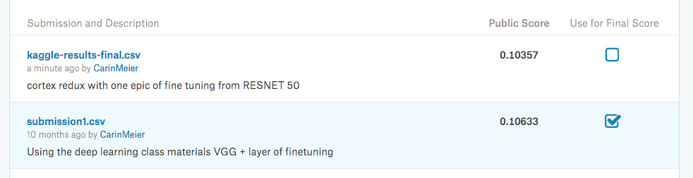
My one epoch of fine tuning beat my best results of going through the Practical Deep Learning exercise with the fine tuning the VGG16 model. Not bad at all.

Summary

For those of you that are interested in checking out the code, it’s out there on github

Even more exciting, there is a walkthrough in a jupyter notebook with a lein-jupyter plugin.

The Deep Learning world in Clojure is an exciting place to be and gaining tools and traction more and more.