
In the last post, we took a look at a simple autoencoder. The autoencoder is a deep learning model that takes in an image and, (through an encoder and decoder), works to produce the same image. In short:
- Autoencoder: image -> image
For a discriminator, we are going to focus on only the first half on the autoencoder.
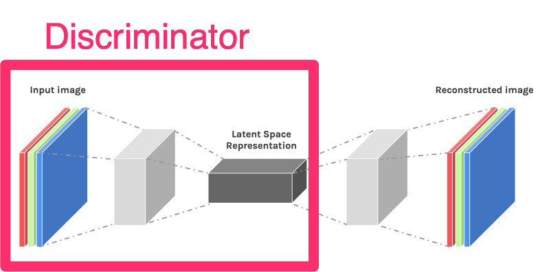
Why only half? We want a different transformation. We are going to want to take an image as input and then do some discrimination of the image and classify what type of image it is. In our case, the model is going to input an image of a handwritten digit and attempt to decide which number it is.
- Discriminator: image -> label
As always, with deep learning. To do anything, we need data.
MNIST Data
Nothing changes here from the autoencoder code. We are still using the MNIST dataset for handwritten digits.
;;; Load the MNIST datasets
(def train-data
  (mx-io/mnist-iter
   {:image (str data-dir "train-images-idx3-ubyte")
    :label (str data-dir "train-labels-idx1-ubyte")
    :input-shape [784]
    :flat true
    :batch-size batch-size
    :shuffle true}))

(def test-data
  (mx-io/mnist-iter
   {:image (str data-dir "t10k-images-idx3-ubyte")
    :label (str data-dir "t10k-labels-idx1-ubyte")
    :input-shape [784]
    :batch-size batch-size
    :flat true
    :shuffle true}))
The model will change since we want a different output.
The Model
We are still taking in the image as input, and using the same encoder layers from the autoencoder model. However, at the end, we use a fully connected layer that has 10 hidden nodes - one for each label of the digits 0-9. Then we use a softmax for the classification output.
(def input (sym/variable "input"))
(def output (sym/variable "input_"))

(defn get-symbol []
  (as-> input data
    ;; encode
    (sym/fully-connected "encode1" {:data data :num-hidden 100})
    (sym/activation "sigmoid1" {:data data :act-type "sigmoid"})

    ;; encode
    (sym/fully-connected "encode2" {:data data :num-hidden 50})
    (sym/activation "sigmoid2" {:data data :act-type "sigmoid"})

    ;;; this last bit changed from autoencoder
    ;;output
    (sym/fully-connected "result" {:data data :num-hidden 10})
    (sym/softmax-output {:data data :label output})))
In the autoencoder, we were never actually using the label, but we will certainly need to use it this time. It is reflected in the model’s bindings with the data and label shapes.
(def model (-> (m/module (get-symbol) {:data-names ["input"] :label-names ["input_"]})
               (m/bind {:data-shapes [(assoc data-desc :name "input")]
                        :label-shapes [(assoc label-desc :name "input_")]})
               (m/init-params {:initializer (initializer/uniform 1)})
               (m/init-optimizer {:optimizer (optimizer/adam {:learning-rage 0.001})})))
For the evaluation metric, we are also going to use an accuracy metric vs a mean squared error (mse) metric
(def my-metric (eval-metric/accuracy))
With these items in place, we are ready to train the model.
Training
The training from the autoencoder needs to changes to use the real label for the the forward pass and updating the metric.
(defn train [num-epochs]
  (doseq [epoch-num (range 0 num-epochs)]
    (println "starting epoch " epoch-num)
    (mx-io/do-batches
     train-data
     (fn [batch]
       ;;; here we make sure to use the label
       ;;; now for forward and update-metric
       (-> model
           (m/forward {:data (mx-io/batch-data batch)
                       :label (mx-io/batch-label batch)})
           (m/update-metric my-metric (mx-io/batch-label batch))
           (m/backward)
           (m/update))))
    (println {:epoch epoch-num
              :metric (eval-metric/get-and-reset my-metric)})))
Let’s Run Things
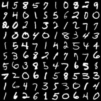
It’s always a good idea to take a look at things before you start training.
The first batch of the training data looks like:
  (def my-batch (mx-io/next train-data))
  (def images (mx-io/batch-data my-batch))
  (viz/im-sav {:title "originals"
               :output-path "results/"
               :x (-> images
                      first
                      (ndarray/reshape [100 1 28 28]))})
Before training, if we take the first batch from the test data and predict what the labels are:
  (def my-test-batch (mx-io/next test-data))
  (def test-images (mx-io/batch-data my-test-batch))
  (viz/im-sav {:title "test-images"
               :output-path "results/"
               :x (-> test-images
                      first
                      (ndarray/reshape [100 1 28 28]))})

  (def preds (m/predict-batch model {:data test-images} ))
  (->> preds
       first
       (ndarray/argmax-channel)
       (ndarray/->vec)
       (take 10))
 ;=> (1.0 8.0 8.0 8.0 8.0 8.0 2.0 8.0 8.0 1.0)
Yeah, not even close. The real first line of the images is 6 1 0 0 3 1 4 8 0 9
Let’s Train!
  (train 3)

;; starting epoch  0
;; {:epoch 0, :metric [accuracy 0.83295]}
;; starting epoch  1
;; {:epoch 1, :metric [accuracy 0.9371333]}
;; starting epoch  2
;; {:epoch 2, :metric [accuracy 0.9547667]}
After the training, let’s have another look at the predicted labels.
  (def preds (m/predict-batch model {:data test-images} ))
  (->> preds
       first
       (ndarray/argmax-channel)
       (ndarray/->vec)
       (take 10))
 ;=> (6.0 1.0 0.0 0.0 3.0 1.0 4.0 8.0 0.0 9.0)
- Predicted =
(6.0 1.0 0.0 0.0 3.0 1.0 4.0 8.0 0.0 9.0) - Actual =
6 1 0 0 3 1 4 8 0 9
Rock on!
Closing
In this post, we focused on the first half of the autoencoder and made a discriminator model that took in an image and gave us a label.
Don’t forget to save the trained model for later, we’ll be using it.
  (m/save-checkpoint model {:prefix "model/discriminator"
                            :epoch 2})
Until then, here is a picture of the cat in a basket to keep you going.

P.S. If you want to run all the code for yourself. It is here