Squid's Blog

A secret message inside a 10,000 hyperdimensional vector

We’ve seen in previous posts how we can encode data structures using Vector Symbolic Architectures in Clojure. This is an exploration of how we can use this to develop a cipher to transmit a secret message between two parties.

A Hyperdimensional Cipher

Usually, we would develop a dictionary/ cleanup memory of randomly chosen hyperdimensional vectors to represent each symbol. We could do this, but then sharing the dictionary as our key to be able to decode messages would be big. Instead, we could share a single hyperdimensional vector and then use the protect/ rotation operator to create a dictionary of the alphabet and some numbers to order the letters. Think of this as the initial seed symbol and the rest being defined as n+1.

1
2
3
4
5
6
7
8
9
10
11
12
13
14
15
16
17
18
19
20

(def alphabet
  [:a :b :c :d :e :f :g :h :i :j :k :l :m :n :o :p :q :r :s :t :u :v :w :x :y :z :end-of-message])


(def max-num 4)
(def numbers (range 1 (inc max-num)))
(def key-codes (into alphabet numbers))


(defn add-keys-to-cleanup-mem!
  "Take a single hdv as a seed and create an alphabet + numbers of them by using rotation/ protect"
  [seed-hdv]
  (vb/reset-hdv-mem!)
  (doall
    (reduce (fn [v k]
              (let [nv (vb/protect v)]
                (vb/add-hdv! k nv)
                nv))
            seed-hdv
            key-codes)))

We can then encode a message by using a VSA data structure map with the form:

1

{1 :c, 2 :a, 3 :t, 4 :s}

where the numbers are the key to the order of the sequence of the message.

1
2
3
4
5
6
7
8
9
10
11

(defn encode-message
  "Encode a message using key value pairs with numbers for ordering"
  [message]
  (when (> (count message) max-num)
    (throw (ex-info "message too long" {:allowed-n max-num})))
  (let [ds (zipmap numbers
                   (conj (->> (mapv str message)
                              (mapv keyword))
                         :end-of-message))]
    (println "Encoding " message " into " ds)
    (vd/clj->vsa ds)))

The message is now in a single hyperdimensional vector. We can decode the message by inspecting each of the numbers in the key value pairs encoded in the data structure.

1
2
3
4
5
6
7
8
9
10
11
12
13
14

(defn decode-message
  "Decode a message by getting the value of the numbered pairs"
  [msg]
  (let [message-v
        _ (println "decoded message-v " message-v)
        decoded (->> message-v
                     (partition-by #(= % :end-of-message))
                     first
                     (mapv #(if (keyword? %)
                              (name %)
                              (str %)))
                     (apply str))]
    (println "Decoded message is " decoded)
    decoded))

Some example code of generating and decoding the message:

1
2
3
4
5
6
7
8
9

  (vb/set-size! 1e4)
  (def seed-key-hdv (vb/hdv))
  (add-keys-to-cleanup-mem! seed-key-hdv)
  (image/write-image-hdv "seed-key-hdv" seed-key-hdv)

  (def message (encode-message "cats"))
  (image/write-image-hdv "secret-message" message)
  (decode-message message)
  ;=> "cats"

The cool thing is that both hyperdimensional dictionary and the hyperdimensional encoded message can both be shared as a simple image like these:

• The seed key to generate the dictionary/ cleanup-mem

• The encoded secret message

Then you can load up the seed key/ message from the image. Once you have the dictionary shared, you can create multiple encoded messages with it.

1
2
3
4

(def loaded-key (image/read-image-to-hdv "examples/seed-key-hdv.png"))
  (add-keys-to-cleanup-mem! loaded-key)
  (def loaded-message (image/read-image-to-hdv "examples/secret-message.png"))
  (decode-message loaded-message)

Caveats

Please keep in mind that this is just an experiment - do not use for anything important. Another interesting factor to keep in mind is that the VSA operations to get the key value are probabilistic so that the correct decoding is not guaranteed. In fact, I set a limit on the 10,000 dimensional vector message to be 4 letters, which I found to be pretty reliable. For example, with 10,000 dimensions, encoding catsz decoded as katsz.

Increasing the number of dimensions lets you encode longer messages. This article is a good companion to look at capacity across different implementations of VSAs.

Conclusion

VSAs could be an interesting way to do ciphers. Some advantages could be that the distribution of the information across the vector and the nature of the mapped data structure, it is hard to do things like vowel counting to try to decipher messages. Of course you don’t need to have letters and numbers be the only symbols used in the dictionary, they could represent other things as well. The simplicity of being able to encode data structures in a form that can easily be expressed as a black and white image, also lends in its flexibility. Another application might be the ability to combine this technique with deep learning to keep information safe during the training process.

Link to the full github code

generated with Stable Diffusion

Before diving into the details of what Vector Symbolic Architectures are and what it means to implement Clojure data structures in them, I’d like to start with some of my motivation in this space.

Small AI for More Personal Enjoyment

Over the last few years, I’ve spent time learning, exploring, and contributing to open source deep learning. It continues to amaze me with its rapid movement and achievements at scale. However, the scale is really too big and too slow for me to enjoy it anymore.

Between work and family, I don’t have a lot of free time. When I do get a few precious hours to do some coding just for me, I want it it to be small enough for me to fire up and play with it in a REPL on my local laptop and get a result back in under two minutes.

I also believe that the current state of AI is not likely to produce any more meaningful revolutionary innovations in the current mainstream deep learning space. This is not to say that there won’t be advances. Just as commercial airlines transformed the original first flight, I’m sure we are going to continue to see the transformation of society with current big models at scale - I just think the next leap forward is going to come from somewhere else. And that somewhere else is going to be small AI.

Vector Symbolic Architures aka Hyperdimensional Computing

Although I’m talking about small AI, VSA or Hyperdimensional computing is based on really big vectors - like 1,000,000 dimensions. The beauty and simplicity in it is that everything is a hypervector - symbols, maps, lists. Through the blessing of high dimensionality, any random hypervector is mathematically guaranteed to be orthogonal to any other one. This all enables some cool things:

• Random hypervectors can be used to represent symbols (like numbers, strings, keywords, etc..)
• We can use an algebra to operate on hypervectors: bundling and binding operations create new hypervectors that are compositions of each other and can store and retrieve key value pairs. These operations furthermore are fuzzy due to the nature of working with vectors. In the following code examples, I will be using the concrete model of MAP (Multiply, Add, Permute) by R. Gayler.
• We can represent Clojure data structures such as maps and vectors in them and perform operations such as get with probabilistic outcomes.
• Everything is a hypervector! I mean you have a keyword that is a symbol that is a hypervector, then you bundle that with other keywords to be a map. The result is a single hypervector. You then create a sequence structure and add some more in. The result is a single hypervector. The simplicity in the algebra and form of the VSA is beautiful - not unlike LISP itself. Actually, P. Kanerva thought that a LISP could be made from it. In my exploration, I only got as far as making some Clojure data structures, but I’m sure it’s possible.

Start with an Intro and a Paper

A good place to start with Vector Symbolic Architectures is actually the paper referenced above - An Introduction to Hyperdimensional Computing for Robots. In general, I find the practice of taking a paper and then trying to implement it a great way to learn.

To work with VSAs in Clojure, I needed a high performing Clojure library with tensors and data types. I reached for https://github.com/techascent/tech.datatype. It could handle a million dimensions pretty easily on my laptop.

To create a new hypervector - simply chose random values between -1 and 1. This gives us a direction in space which is enough.

1
2
3
4
5
6
7
8
9
10
11
12
13
14

;; Uses Gaylor Method for HDV Operations

(def size 1e6)  ; big enough for the "Blessing of Dimensionality"

(defn binary-rand
  "Choose a random binary magnitude for the vector +1 or -1"
  []
  (if (> (rand) 0.5) -1 1))


(defn hdv
  "Create a random hyperdimensional vector of default size"
  []
  (dtt/->tensor (repeatedly size #(binary-rand)) :datatype :int8))

The only main operations to create key value pairs is addition and matrix multiplication.

Adding two hyperdimensional vectors, (hdvs), together is calling bundling. Note we clip the values to 1 or -1. At high dimensions, only the direction really matters not the magnitude.

1
2
3
4
5
6
7
8
9
10
11
12
13
14
15

(defn clip
  "Clips the hyperdimensional vector magnitude to 1 or -1.
   We can discard these because of the nature of the large vectors
   that the mangitudes do not matter"
  [v]
  (-> v
      (dtype-fn/min 1)
      (dtype-fn/max -1)))


(defn bundle
  "Adds two hyperdimensional vectors together into a single bundle"
  [v1 v2]
  (-> (bundle-op v1 v2)
      (clip)))

We can assign key values using bind which is matrix multiplication.

1
2
3
4

(defn bind
  "Binds two HDVs using the multiplication operator. This binding is akin to assigning a symbol to a value. "
  [v1 v2]
  (dtype-fn/* v1 v2))

One cool thing is that the binding of a key value pair is also the inverse of itself. So to unbind is just to bind again.

The final thing we need is a cleanup memory. The purpose of this is to store the hdv somewhere without any noise. As the hdv gets bundled with other operations there is noise associated with it. It helps to use the cleaned up version by comparing the result to the memory version for future operations. For Clojure, this can be a simple atom.

Following along the example in the paper, we reset the cleanup memory and add some symbols.

1
2
3
4
5
6
7
8

(vb/reset-hdv-mem!)

(vb/add-hdv! :name)
(vb/add-hdv! "Alice")
(vb/add-hdv! :yob)
(vb/add-hdv! 1980)
(vb/add-hdv! :high-score)
(vb/add-hdv! 1000)

Next we create the key value map with combinations of bind and bundle.

1
2
3
4
5
6

(def H
  (-> (vb/bind (vb/get-hdv :name) (vb/get-hdv "Alice"))
      (vb/bundle
        (vb/bind (vb/get-hdv :yob) (vb/get-hdv 1980)))
      (vb/bundle
        (vb/bind (vb/get-hdv :high-score) (vb/get-hdv 1000)))))

So H is just one hypervector as a result of this. We can then query it. unbind-get is using the bind operation as inverse. So if we want to query for the :name value, we get the :name hdv from memory and do the bind operation on the H data structure which is the inverse.

1
2
3
4
5

(vb/unbind-get H :name)


;; ["Alice" #tech.v3.tensor<int8>[1000000]
;;  [-1 1 1 ... 1 -1 -1]]

We can find other values like :high-score.

1
2
3
4
5

(vb/unbind-get H :high-score)


;;  [1000 #tech.v3.tensor<int8>[1000000]
;; [-1 -1 1 ... -1 1 1]]

Or go the other way and look for Alice.

1
2
3
4
5

(vb/unbind-get H "Alice")


;; [:name #tech.v3.tensor<int8>[1000000]
;; [-1 1 -1 ... -1 -1 -1]]

Now that we have the fundamentals from the paper, we can try to implement some Clojure data structures.

Clojure Data Structures in VSAs

First things first, let’s clear our cleanup memory.

1

(vb/reset-hdv-mem!)

Let’s start off with a map, (keeping to non-nested versions to keep things simple).

1

(def our-first-vsa-map (vd/clj->vsa {:x 1 :y 2}))

The result is a 1,000,000 dimension hypervector - but remember all the parts are also hypervectors as well. Let’s take a look at what is in the cleanup memory so far.

1
2
3
4
5
6
7

@vb/cleanup-mem


;; {:x #tech.v3.tensor<int8>[1000000][1 -1 1 ... 1 -1 -1],
;;  1 #tech.v3.tensor<int8>[1000000][1 1 -1 ... -1 -1 -1],
;;  :y #tech.v3.tensor<int8>[1000000][1 1 -1 ... 1 1 1],
;;  2 #tech.v3.tensor<int8>[1000000][-1 -1 -1 ... -1 -1 1]}

We can write a vsa-get function that takes the composite hypervector of the map and get the value from it by finding the closest match with cosine similarity to the cleanup memory.

1
2
3
4

(vd/vsa-get our-first-vsa-map :x)


;; =>  [1 #tech.v3.tensor<int8>[1000000][1 1 -1 ... -1 -1 -1]

In the example above, the symbolic value is the first item in the vector, in this case the number 1, and the actual hypervector is the second value.

We can add onto the map with a new key value pair.

1
2
3
4
5
6

(def our-second-vsa-map (vd/vsa-assoc our-first-vsa-map :z 3))

(vd/vsa-get our-second-vsa-map :z)


;; =>  [3 #tech.v3.tensor<int8>[1000000][1 -1 1 ... -1 -1 1]]

We can represent Clojure vectors as VSA data structures as well by using the permute (or rotate) and adding them like a stack.

1
2
3
4
5
6
7
8
9
10
11
12
13
14

(def our-first-vsa-vector-of-maps (vd/clj->vsa [{:x 1} {:x 2 :y 3}]))


;; We can get the value of x in the 2nd map by
(vd/vsa-get our-first-vsa-vector-of-maps :x {:idx 1})


;; [2 #tech.v3.tensor<int8>[1000000][-1 1 1 ... 1 -1 1]]

;; Or the first map
(vd/vsa-get our-first-vsa-vector-of-maps :x {:idx 0})


;; =>  [1 #tech.v3.tensor<int8>[1000000][-1 -1 1 ... 1 1 1]]

We can also add onto the Clojure vector with a conj.

1
2
3
4
5
6
7
8

(def our-second-vsa-vector-of-maps
  (vd/vsa-conj our-first-vsa-vector-of-maps (vd/clj->vsa {:z 5})))


(vd/vsa-get our-second-vsa-vector-of-maps :z {:idx 2})


;; =>  [5 #tech.v3.tensor<int8>[1000000][-1 1 1 ... -1 -1 -1]]

What is really cool about this is that we have built in fuzziness or similarity matching. For example, with this map, we have more than one possibility of matching.

1

(def vsa-simple-map (vd/clj->vsa {:x 1 :y 1 :z 3}))

We can see all the possible matches and scores

1
2
3
4
5
6
7
8
9

(vd/vsa-get vsa-simple-map :x {:threshold -1 :verbose? true})


;; =>  [{1 #tech.v3.tensor<int8>[1000000]
;;      [1 -1 1 ... -1 -1 -1], :dot 125165.0, :cos-sim 0.1582533568106879}  {:x #tech.v3.tensor<int8>[1000000]
;;      [1 -1 -1 ... -1 -1 1], :dot 2493.0, :cos-sim 0.0031520442498225933} {:z #tech.v3.tensor<int8>[1000000]
;;      [-1 -1 1 ... 1 1 -1], :dot 439.0, :cos-sim 5.550531190020531E-4}    {3 #tech.v3.tensor<int8>[1000000]
;;      [-1 -1 1 ... -1 -1 1], :dot -443.0, :cos-sim -5.601105506102723E-4}  {:y #tech.v3.tensor<int8>[1000000]
;;      [-1 -1 1 ... 1 1 1], :dot -751.0, :cos-sim -9.495327844431478E-4}]

This opens up the possibility of defining compound symbolic values and doing fuzzy matching. For example with colors.

1
2
3

(vb/reset-hdv-mem!)

(def primary-color-vsa-map (vd/clj->vsa {:x :red :y :yellow :z :blue}))

Let’s add a new compound value to the cleanup memory that is green based on yellow and blue.

1
2
3

(vb/add-hdv! :green (vb/bundle
                      (vb/get-hdv :yellow)
                      (vb/get-hdv :blue)))

Now we can query the hdv color map for things that are close to green.

1
2
3
4
5

(vd/vsa-get primary-color-vsa-map :green {:threshold 0.1})


;; =>  [{:z #tech.v3.tensor<int8>[1000000][1 -1 1 ... -1 1 1]}
;;     {:y #tech.v3.tensor<int8>[1000000] [-1 1 1 ... 1 1 1]}]

We can also define an inspect function for a hdv by comparing the similarity of all the values of the cleanup memory in it.

1
2
3
4
5
6
7
8
9
10

(vd/vsa-inspect primary-color-vsa-map)


;; Note that it includes green in it since it is a compound value
;; =>  #{:y :yellow :green :z :red :blue :x}

(vd/vsa-inspect (vd/clj->vsa {:x :red}))


;; =>  #{:red :x}

Finally, we can implement clojure map and filter functions on the vector data structures that can also include fuzziness.

1
2
3
4
5
6
7
8
9
10
11
12
13
14
15
16
17

(def color-vsa-vector-map (vd/clj->vsa [{:x :yellow} {:x :green} {:z :red}]))


(vd/vsa-map #(->> (vd/vsa-get % :yellow {:threshold 0.01})
                  (mapv ffirst))
            color-vsa-vector-map)


;; =>  ([:x] [:x] [])


(->> color-vsa-vector-map
     (vd/vsa-filter #(vd/vsa-get % :yellow {:threshold 0.01}))
     count)


;; =>  2

Wrap Up

VSAs and hyperdimensional computing seem like a natural fit for LISP and Clojure. I’ve only scratched the surface here in how the two can fit together. I hope that more people are inspired to look into it and small AI with big dimensions.

Full code and examples here https://github.com/gigasquid/vsa-clj.

Special thanks to Ross Gayler in helping me to implement VSAs and understanding their coolness.

What if I told you that you could pick up a library model and instantly classify text with arbitrary categories without any training or fine tuning?

That is exactly what we are going to do with Hugging Face’s zero-shot learning model. We will also be using libpython-clj to do this exploration without leaving the comfort of our trusty Clojure REPL.

What’s for breakfast?

We’ll start off by taking some text from a recipe description and trying to decide if it’s for breakfast, lunch or dinner:

"French Toast with egg and bacon in the center with maple syrup on top. Sprinkle with powdered sugar if desired."

Next we will need to install the required python deps:

pip install numpy torch transformers lime

Now we just need to set up the libpython clojure namespace to load the Hugging Face transformers library.

1
2
3
4
5
6
7

(ns gigasquid.zeroshot
  (:require
   [libpython-clj2.python :as py :refer [py. py.. py.-]]
   [libpython-clj2.require :refer [require-python]]))


(require-python '[transformers :bind-ns])

Setup is complete. We are now ready to classify with zeroshot.

Classify with Zero Shot

To create the classifier with zero shot, you need only create it with a handy pipeline function.

1

(def classifier (py. transformers "pipeline" "zero-shot-classification"))

After that you need just the text you want to classify and category labels you want to use.

1
2
3

(def text "French Toast with egg and bacon in the center with maple syrup on top. Sprinkle with powdered sugar if desired.")

(def labels ["breakfast" "lunch" "dinner"])

Classification is only a function call away with:

1
2
3
4

(classifier text labels)

{'labels': ['breakfast', 'lunch', 'dinner'],
 'scores': [0.989736795425415, 0.007010194938629866, 0.003252972150221467]}

Breakfast is the winner. Notice that all the probabilities add up to 1. This is because the default mode for classify uses softmax. We can change that so the categories are each considered independently with the :multi-class option.

1
2
3

(classifier text labels :multi_class true)
{'labels': ['breakfast', 'lunch', 'dinner'],
 'scores': [0.9959920048713684, 0.22608685493469238, 0.031050905585289]}

This is a really powerful technique for such an easy to use library. However, how can we do anything with it if we don’t understand how it is working and get a handle on how to debug it. We need some level of trust in it for utility.

This is where LIME enters.

Using LIME for Interpretable Models

One of the biggest problems holding back applying state of the art machine learning models to real life problems is that of interpretability and trust. The lime technique is a well designed tool to help with this. One of the reasons that I really like it is that it is model agnostic. This means that you can use it with whatever code you want to use with it as long as you adhere to it’s api. You need to provide it with the input and a function that will classify and return the probabilities in a numpy array.

The creation of the explainer is only a require away:

1
2
3
4
5

(require-python '[lime.lime_text :as lime])
(require-python 'numpy)


(def explainer (lime/LimeTextExplainer :class_names labels))

We need to create a function that will take in some text and then return the probabilities for the labels. Since the zeroshot classifier will reorder the returning labels/probs by the value, we need to make sure that it will match up by index to the original labels.

1
2
3
4
5
6
7
8
9
10
11
12
13
14
15
16
17
18

(defn predict-probs
  [text]
  (let [result (classifier text labels)
        result-scores (get result "scores")
        result-labels (get result "labels")
        result-map (zipmap result-labels result-scores)]
    (mapv (fn [cn]
            (get result-map cn))
          labels)))


(defn predict-texts
  [texts]
  (println "lime texts are " texts)
  (numpy/array (mapv predict-probs texts)))


 (predict-texts [text]) ;=>  [[0.99718672 0.00281324]]

Finally we make an explanation for our text here. We are only using 6 features and 100 samples, to keep the cpus down, but in real life you would want to use closer to the default amount of 5000 samples. The samples are how the explainers work, it modifies the text over and over again and sees the difference in classification values. For example, one of the sample texts for our case is ' Toast with bacon in the center with syrup on . with sugar desired.'.

1
2
3
4
5
6
7

(def exp-result
  (py. explainer "explain_instance" text predict-texts
       :num_features 6
       :num_samples 100))


(py. exp-result "save_to_file" "explanation.html")

Now it becomes more clear. The model is using mainly the word toast to classify it as breakfast with supporting words also being french, egg, maple, and syrup. The word the is also in there too which could be an artifact of the low numbers of samples we used or not. But now at least we have the tools to dig in and understand.

Final Thoughts

Exciting advances are happening in Deep Learning and NLP. To make them truly useful, we will need to continue to consider how to make them interpretable and debuggable.

As always, keep your Clojure REPL handy.

AI Debate 2 from Montreal.AI

I had the pleasure of watching the second AI debate from Montreal.AI last night. The first AI debate occurred last year between Yoshua Bengio and Gary Marcus entitled “The Best Way Forward for AI” in which Yoshua argued that Deep Learning could achieve General AI through its own paradigm, while Marcus argued that Deep Learning alone was not sufficient and needed a hybrid approach involving symbolics and inspiration from other disciplines.

This interdisciplinary thread of Gary’s linked the two programs. The second AI debate was entitled “Moving AI Forward: An Interdisciplinary Approach” and reflected a broad panel that explored themes on architecture, neuroscience and psychology, and trust/ethics. The second program was not really a debate, but more of a showcase of ideas in the form of 3 minute presentations from the panelists and discussion around topics with Marcus serving as a capable moderator.

The program aired Wednesday night and was 3 hours long. I watched it live with an unavoidable break in the middle to fetch dinner for my family, but the whole recording is up now on the website. Some of the highlights for me were thoughts around System 1 and System 2, reinforcement learning, and the properties of evolution.

There was much discussion around System 1 and System 2 in relation to AI. One of the author’s of the recently published paper “Thinking Fast and Slow in AI”, Francesca Rossi was a panelist as well as Danny Kahneman the author of “Thinking Fast and Slow”. Applying the abstraction of these sysems to AI with Deep Learning being System 1 is very appealing, however as Kahneman pointed out in his talk, this abstraction is leaky at its heart as the human System 1 encompasses much more than current AI system 1, (like a model of the world). It is interesting to think of one of the differences in human System 1 and System 2 in relation to one being fast and concurrent while the other is slower and sequential and laden with attention. Why is this so? Is this a constraint and design feature that we should bring to our AI design?

Richard Sutton gave a thought provoking talk on how reinforcement learning is the first fully implemented computational theory of intelligence. He pointed to Marr’s three levels at which any information processing machine must be understood: hardware implementation, representation/algorithm, and finally the high level theory. That is: what is the goal of the computation? What logic can the strategy be carried out? AI has made great strides due to this computational theory. However, it is only one theory. We need more. I personally think that innovation and exploration in this area could lead to an exciting future in AI.

Evolution is a fundamental force that drives humans and the world around us. Ken Stanely reminded us that while computers dominate at solving problems, humans still rule at open-ended innovation over the millenia. The underlying properties of evolution still elude our deep understanding. Studying the core nature of this powerful phenomena is a very important area of research.

The last question of the evening to all the panelists was the greatest Christmas gift of all - “Where do you want AI to go?”. The diversity of the answers reflected the broad hopes shared by many that will light the way to come. I’ll paraphrase some of the ones here:

• Want to understand fundamental laws and principles and use them to better the human condition.
• Understand the different varieties of intelligence.
• Want an intelligent and superfriendly apprentice. To understand self by emulating.
• To move beyond GPT-3 remixing to really assisting creativity for humanity.
• Hope that AI will amplify us and our abilities.
• Use AI to help people understand what bias they have.
• That humans will still have something to add after AI have mastered a domain
• To understand the brain in the most simple and beautiful way.
• Gain a better clarity and understanding of our own values by deciding which to endow our AI with.
• Want the costs and benefits of AI to be distributed globally and economically.

Thanks again Montreal.AI for putting together such a great program and sharing it with the community. I look forward to next year.

Merry Christmas everyone!

In this edition of the blog series of Clojure/Python interop with libpython-clj, we’ll be taking a look at two popular Python NLP libraries: NLTK and SpaCy.

NLTK - Natural Language Toolkit

I was taking requests for doing examples of python-clojure interop libraries on twitter the other day, and by far NLTK was the most requested library. After looking into it, I can see why. It’s the most popular natural language processing library in Python and you will see it everywhere there is text someone is touching.

Installation

To use the NLTK toolkit you will need to install it. I use sudo pip3 install nltk, but libpython-clj now supports virtual environments with this PR, so feel free to use whatever is best for you.

Features

We’ll take a quick tour of the features of NLTK following along initially with the nltk official book and then moving onto this more data task centered tutorial.

First, we need to require all of our things as usual:

1
2
3
4

(ns gigasquid.nltk
  (:require [libpython-clj.require :refer [require-python]]
            [libpython-clj.python :as py :refer [py. py.. py.-]]))
(require-python '([nltk :as nltk]))

Downloading packages

There are all sorts of packages available to download from NLTK. To start out and tour the library, I would go with a small one that has basic data for the nltk book tutorial.

1
2

 (nltk/download "book")
  (require-python '([nltk.book :as book]))

There are all other sorts of downloads as well, such as (nltk/download "popular") for most used ones. You can also download "all", but beware that it is big.

You can check out some of the texts it downloaded with:

1
2
3
4
5
6
7
8
9
10
11
12
13
14
15
16

  (book/texts)

  ;;; prints out in repl
  ;; text1: Moby Dick by Herman Melville 1851
  ;; text2: Sense and Sensibility by Jane Austen 1811
  ;; text3: The Book of Genesis
  ;; text4: Inaugural Address Corpus
  ;; text5: Chat Corpus
  ;; text6: Monty Python and the Holy Grail
  ;; text7: Wall Street Journal
  ;; text8: Personals Corpus
  ;; text9: The Man Who Was Thursday by G . K . Chesterton 1908

  book/text1 ;=>  <Text: Moby Dick by Herman Melville 1851>
  book/text2 ;=>  <Text: Sense and Sensibility by Jane Austen 1811>

You can do fun things like see how many tokens are in a text

1

  (count (py.- book/text3 tokens))  ;=> 44764

Or even see the lexical diversity, which is a measure of the richness of the text by looking at the unique set of word tokens against the total tokens.

1
2
3
4
5
6
7

  (defn lexical-diversity [text]
    (let [tokens (py.- text tokens)]
      (/ (-> tokens set count)
         (* 1.0 (count tokens)))))

  (lexical-diversity book/text3) ;=> 0.06230453042623537
  (lexical-diversity book/text5) ;=> 0.13477005109975562

This of course is all very interesting but I prefer to look at some more practical tasks, so we are going to look at some sentence tokenization.

Sentence Tokenization

Text can be broken up into individual word tokens or sentence tokens. Let’s start off first with the token package

1
2
3

(require-python '([nltk.tokenize :as tokenize]))
(def text "Hello Mr. Smith, how are you doing today? The weather is great, and city is awesome.
The sky is pinkish-blue. You shouldn't eat cardboard")

To tokenize sentences, you take the text and use tokenize/sent_tokenize.

1
2
3
4
5

 (def text "Hello Mr. Smith, how are you doing today? The weather is great, and city is awesome.
The sky is pinkish-blue. You shouldn't eat cardboard")
 (def tokenized-sent (tokenize/sent_tokenize text))
 tokenized-sent
 ;;=> ['Hello Mr. Smith, how are you doing today?', 'The weather is great, and city is awesome.', 'The sky is pinkish-blue.', "You shouldn't eat cardboard"]

Likewise, to tokenize words, you use tokenize/word_tokenize:

1
2
3
4
5
6
7
8
9
10

 (def text "Hello Mr. Smith, how are you doing today? The weather is great, and city is awesome.
The sky is pinkish-blue. You shouldn't eat cardboard")
 (def tokenized-sent (tokenize/sent_tokenize text))
 tokenized-sent
 ;;=> ['Hello Mr. Smith, how are you doing today?', 'The weather is great, and city is awesome.', 'The sky is pinkish-blue.', "You shouldn't eat cardboard"]


 (def tokenized-word (tokenize/word_tokenize text))
 tokenized-word
  ;;=> ['Hello', 'Mr.', 'Smith', ',', 'how', 'are', 'you', 'doing', 'today', '?', 'The', 'weather', 'is', 'great', ',', 'and', 'city', 'is', 'awesome', '.', 'The', 'sky', 'is', 'pinkish-blue', '.', 'You', 'should', "n't", 'eat', 'cardboard']

Frequency Distribution

You can also look at the frequency distribution of the words with using the probability package.

1
2
3
4
5
6
7

 (require-python '([nltk.probability :as probability]))

 (def fdist (probability/FreqDist tokenized-word))
 fdist ;=> <FreqDist with 25 samples and 30 outcomes>

 (py. fdist most_common)
  ;=> [('is', 3), (',', 2), ('The', 2), ('.', 2), ('Hello', 1), ('Mr.', 1), ('Smith', 1), ('how', 1), ('are', 1), ('you', 1), ('doing', 1), ('today', 1), ('?', 1), ('weather', 1), ('great', 1), ('and', 1), ('city', 1), ('awesome', 1), ('sky', 1), ('pinkish-blue', 1), ('You', 1), ('should', 1), ("n't", 1), ('eat', 1), ('cardboard', 1)]

Stop Words

Stop words are considered noise in text and there are ways to use the library to remove them using the nltk.corpus.

1
2
3

(def stop-words (into #{} (py. corpus/stopwords words "english")))
 stop-words
  ;=> #{"d" "itself" "more" "didn't" "ain" "won" "hers"....}

Now that we have a collection of the stop words, we can filter them out of our text in the normal way in Clojure.

1
2
3
4
5
6
7
8

(def filtered-sent (->> tokenized-sent
                         (map tokenize/word_tokenize)
                         (map #(remove stop-words %))))
 filtered-sent
 ;; (("Hello" "Mr." "Smith" "," "today" "?")
 ;; ("The" "weather" "great" "," "city" "awesome" ".")
 ;; ("The" "sky" "pinkish-blue" ".")
 ;; ("You" "n't" "eat" "cardboard"))

Lexion Normalization and Lemmatization

Stemming and Lemmatization allow ways for the text to be reduced to base words and normalized. For example, the word flying has a stemmed word of fli and a lemma of fly.

1
2
3
4
5
6
7
8
9

(require-python '([nltk.stem :as stem]))
(require-python '([nltk.stem.wordnet :as wordnet]))

(let [lem (wordnet/WordNetLemmatizer)
       stem (stem/PorterStemmer)
       word "flying"]
   {:lemmatized-word (py. lem lemmatize word "v")
    :stemmed-word (py. stem stem word)})
 ;=> {:lemmatized-word "fly", :stemmed-word "fli"}

POS Tagging

It also has support for Part-of-Speech (POS) Tagging. A quick example of that is:

1
2
3
4
5
6
7
8

(let [sent "Albert Einstein was born in Ulm, Germany in 1879."
       tokens (nltk/word_tokenize sent)]
   {:tokens tokens
    :pos-tag (nltk/pos_tag tokens)})
 ;; {:tokens
 ;; ['Albert', 'Einstein', 'was', 'born', 'in', 'Ulm', ',', 'Germany', 'in', '1879', '.'],
 ;; :pos-tag
 ;; [('Albert', 'NNP'), ('Einstein', 'NNP'), ('was', 'VBD'), ('born', 'VBN'), ('in', 'IN'), ('Ulm', 'NNP'), (',', ','), ('Germany', 'NNP'), ('in', 'IN'), ('1879', 'CD'), ('.', '.')]}

Phew! That’s a brief overview of what NLTK can do, now what about the other library SpaCy?

SpaCy

SpaCy is the main competitor to NLTK. It has a more opinionated library which is more object oriented than NLTK which mainly processes text. It has better performance for tokenization and POS tagging and has support for word vectors, which NLTK does not.

Let’s dive in a take a look at it.

Installation

To install spaCy, you will need to do:

• pip3 install spacy
• python3 -m spacy download en_core_web_sm to load up the small language model

We’ll be following along this tutorial

We will, of course, need to load up the library

1

(require-python '([spacy :as spacy]))

and its language model:

1

(def nlp (spacy/load "en_core_web_sm"))

Linguistic Annotations

There are many linguistic annotations that are available, from POS, lemmas, and more:

1
2
3
4
5
6
7
8
9
10
11
12
13
14
15

(let [doc (nlp "Apple is looking at buying U.K. startup for $1 billion")]
  (map (fn [token]
         [(py.- token text) (py.- token pos_) (py.- token dep_)])
       doc))
;; (["Apple" "PROPN" "nsubj"]
;;  ["is" "AUX" "aux"]
;;  ["looking" "VERB" "ROOT"]
;;  ["at" "ADP" "prep"]
;;  ["buying" "VERB" "pcomp"]
;;  ["U.K." "PROPN" "compound"]
;;  ["startup" "NOUN" "dobj"]
;;  ["for" "ADP" "prep"]
;;  ["$" "SYM" "quantmod"]
;;  ["1" "NUM" "compound"]
;;  ["billion" "NUM" "pobj"])

Here are some more:

1
2
3
4
5
6
7
8
9
10
11
12
13
14
15
16
17
18
19
20
21
22
23
24
25
26
27
28
29

(let [doc (nlp "Apple is looking at buying U.K. startup for $1 billion")]
  (map (fn [token]
         {:text (py.- token text)
          :lemma (py.- token lemma_)
          :pos (py.- token pos_)
          :tag (py.- token tag_)
          :dep (py.- token dep_)
          :shape (py.- token shape_)
          :alpha (py.- token is_alpha)
          :is_stop (py.- token is_stop)} )
       doc))

;; ({:text "Apple",
;;   :lemma "Apple",
;;   :pos "PROPN",
;;   :tag "NNP",
;;   :dep "nsubj",
;;   :shape "Xxxxx",
;;   :alpha true,
;;   :is_stop false}
;;  {:text "is",
;;   :lemma "be",
;;   :pos "AUX",
;;   :tag "VBZ",
;;   :dep "aux",
;;   :shape "xx",
;;   :alpha true,
;;   :is_stop true}
;;  ...

Named Entities

It also handles named entities in the same fashion.

1
2
3
4
5
6
7
8
9
10
11

(let [doc (nlp "Apple is looking at buying U.K. startup for $1 billion")]
  (map (fn [ent]
         {:text (py.- ent text)
          :start-char (py.- ent start_char)
          :end-char (py.- ent end_char)
          :label (py.- ent label_)} )
       (py.- doc ents)))

;; ({:text "Apple", :start-char 0, :end-char 5, :label "ORG"}
;;  {:text "U.K.", :start-char 27, :end-char 31, :label "GPE"}
;;  {:text "$1 billion", :start-char 44, :end-char 54, :label "MONEY"})

As you can see, it can handle pretty much the same things as NLTK. But let’s take a look at what it can do that NLTK and that is with word vectors.

Word Vectors

In order to use word vectors, you will have to load up a medium or large size data model because the small ones don’t ship with word vectors. You can do that at the command line with:

1

python3 -m spacy download en_core_web_md

You will need to restart your repl and then load it with:

1
2

(require-python '([spacy :as spacy]))
(def nlp (spacy/load "en_core_web_md"))

Now you can see cool word vector stuff!

1
2
3
4
5
6
7
8
9
10
11
12
13
14
15
16
17
18
19
20
21

(let [tokens (nlp "dog cat banana afskfsd")]
  (map (fn [token]
         {:text (py.- token text)
          :has-vector (py.- token has_vector)
          :vector_norm (py.- token vector_norm)
          :is_oov (py.- token is_oov)} )
       tokens))

;; ({:text "dog",
;;   :has-vector true,
;;   :vector_norm 7.033673286437988,
;;   :is_oov false}
;;  {:text "cat",
;;   :has-vector true,
;;   :vector_norm 6.680818557739258,
;;   :is_oov false}
;;  {:text "banana",
;;   :has-vector true,
;;   :vector_norm 6.700014114379883,
;;   :is_oov false}
;;  {:text "afskfsd", :has-vector false, :vector_norm 0.0, :is_oov true})

And find similarity between different words.

1
2
3
4
5
6
7
8
9
10
11
12
13
14
15
16

(let [tokens (nlp "dog cat banana")]
  (for [token1 tokens
        token2 tokens]
    {:token1 (py.- token1 text)
     :token2 (py.- token2 text)
     :similarity (py. token1 similarity token2)}))

;; ({:token1 "dog", :token2 "dog", :similarity 1.0}
;;  {:token1 "dog", :token2 "cat", :similarity 0.8016854524612427}
;;  {:token1 "dog", :token2 "banana", :similarity 0.2432764321565628}
;;  {:token1 "cat", :token2 "dog", :similarity 0.8016854524612427}
;;  {:token1 "cat", :token2 "cat", :similarity 1.0}
;;  {:token1 "cat", :token2 "banana", :similarity 0.28154364228248596}
;;  {:token1 "banana", :token2 "dog", :similarity 0.2432764321565628}
;;  {:token1 "banana", :token2 "cat", :similarity 0.28154364228248596}
;;  {:token1 "banana", :token2 "banana", :similarity 1.0})

Wrap up

We’ve seen a grand tour of the two most popular natural language python libraries that you can now use through Clojure interop!

I hope you’ve enjoyed it and if you are interested in exploring yourself, the code examples are here

libpython-clj has opened the door for Clojure to directly interop with Python libraries. That means we can take just about any Python library and directly use it in our Clojure REPL. But what about matplotlib?

Matplotlib.pyplot is a standard fixture in most tutorials and python data science code. How do we interop with a python graphics library?

How do you interop?

It turns out that matplotlib has a headless mode where we can export the graphics and then display it using any method that we would normally use to display a .png file. In my case, I made a quick macro for it using the shell open. I’m sure that someone out that could improve upon it, (and maybe even make it a cool utility lib), but it suits what I’m doing so far:

1
2
3
4
5
6
7
8
9
10
11
12
13
14
15
16
17
18
19
20
21
22
23
24
25
26
27
28

ns gigasquid.plot
(:require [libpython-clj.require :refer [require-python]]
[libpython-clj.python :as py :refer [py. py.. py.-]]
[clojure.java.shell :as sh])


;;; This uses the headless version of matplotlib to generate a graph then copy it to the JVM
;; where we can then print it

;;;; have to set the headless mode before requiring pyplot
(def mplt (py/import-module "matplotlib"))
(py. mplt "use" "Agg")

(require-python 'matplotlib.pyplot)
(require-python 'matplotlib.backends.backend_agg)
(require-python 'numpy)


(defmacro with-show
  "Takes forms with mathplotlib.pyplot to then show locally"
  [& body]
  `(let [_# (matplotlib.pyplot/clf)
         fig# (matplotlib.pyplot/figure)
         agg-canvas# (matplotlib.backends.backend_agg/FigureCanvasAgg fig#)]
     ~(cons 'do body)
     (py. agg-canvas# "draw")
     (matplotlib.pyplot/savefig "temp.png")
     (sh/sh "open" "temp.png")))

Parens for Pyplot!

Now that we have our wrapper let’s take it for a spin. We’ll be following along more or less this tutorial for numpy plotting

For setup you will need the following installed in your python environment:

• numpy
• matplotlib
• pillow

We are also going to use the latest and greatest syntax from libpython-clj so you are going to need to install the snapshot version locally until the next version goes out:

• git clone git@github.com:cnuernber/libpython-clj.git
• cd cd libpython-clj
• lein install

After that is all setup we can require the libs we need in clojure.

1
2
3
4

(ns gigasquid.numpy-plot
  (:require [libpython-clj.require :refer [require-python]]
            [libpython-clj.python :as py :refer [py. py.. py.-]]
            [gigasquid.plot :as plot]))

The plot namespace contains the macro for with-show above. The py. and others is the new and improved syntax for interop.

Simple Sin and Cos

Let’s start off with a simple sine and cosine functions. This code will create a x numpy vector of a range from 0 to 3 * pi in 0.1 increments and then create y numpy vector of the sin of that and plot it

1
2
3
4

(let [x (numpy/arange 0 (* 3 numpy/pi) 0.1)
        y (numpy/sin x)]
    (plot/with-show
      (matplotlib.pyplot/plot x y)))

Beautiful yes!

Let’s get a bit more complicated now and and plot both the sin and cosine as well as add labels, title, and legend.

1
2
3
4
5
6
7
8
9
10

(let [x (numpy/arange 0 (* 3 numpy/pi) 0.1)
        y-sin (numpy/sin x)
        y-cos (numpy/cos x)]
    (plot/with-show
      (matplotlib.pyplot/plot x y-sin)
      (matplotlib.pyplot/plot x y-cos)
      (matplotlib.pyplot/xlabel "x axis label")
      (matplotlib.pyplot/ylabel "y axis label")
      (matplotlib.pyplot/title "Sine and Cosine")
      (matplotlib.pyplot/legend ["Sine" "Cosine"])))

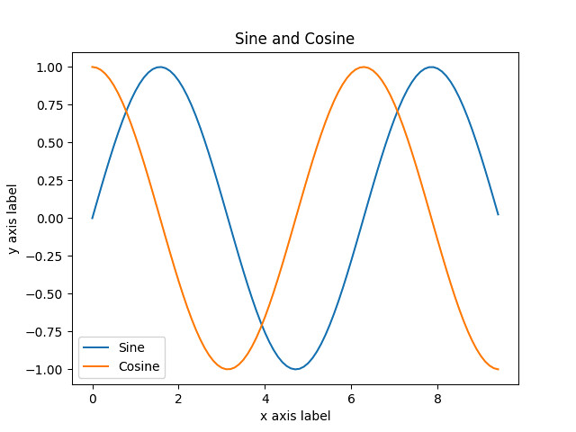
We can also add subplots. Subplots are when you divide the plots into different portions. It is a bit stateful and involves making one subplot active and making changes and then making the other subplot active. Again not too hard to do with Clojure.

1
2
3
4
5
6
7
8
9
10
11
12
13
14

(let [x (numpy/arange 0 (* 3 numpy/pi) 0.1)
        y-sin (numpy/sin x)
        y-cos (numpy/cos x)]
    (plot/with-show
      ;;; set up a subplot gird that has a height of 2 and width of 1
      ;; and set the first such subplot as active
      (matplotlib.pyplot/subplot 2 1 1)
      (matplotlib.pyplot/plot x y-sin)
      (matplotlib.pyplot/title "Sine")

      ;;; set the second subplot as active and make the second plot
      (matplotlib.pyplot/subplot 2 1 2)
      (matplotlib.pyplot/plot x y-cos)
      (matplotlib.pyplot/title "Cosine")))

Plotting with Images

Pyplot also has functions for working directly with images as well. Here we take a picture of my cat and create another version of it that is tinted.

1
2
3
4
5
6
7

(let [img (matplotlib.pyplot/imread "resources/cat.jpg")
        img-tinted (numpy/multiply img [1 0.95 0.9])]
    (plot/with-show
      (matplotlib.pyplot/subplot 1 2 1)
      (matplotlib.pyplot/imshow img)
      (matplotlib.pyplot/subplot 1 2 2)
      (matplotlib.pyplot/imshow (numpy/uint8 img-tinted))))

Pie charts

Finally, we can show how to do a pie chart. I asked people in a twitter thread what they wanted an example of in python interop and one of them was a pie chart. This is for you!

The original code for this example came from this tutorial.

1
2
3
4
5
6
7
8
9
10

(let [labels ["Frogs" "Hogs" "Dogs" "Logs"]
        sizes [15 30 45 10]
        explode [0 0.1 0 0] ; only explode the 2nd slice (Hogs)
        ]
    (plot/with-show
      (let [[fig1 ax1] (matplotlib.pyplot/subplots)]
        (py. ax1 "pie" sizes :explode explode :labels labels :autopct "%1.1f%%"
                             :shadow true :startangle 90)
        (py. ax1 "axis" "equal")) ;equal aspec ration ensures that pie is drawn as circle
      ))

Onwards and Upwards!

This is just the beginning. In upcoming posts, I will be showcasing examples of interop with different libraries from the python ecosystem. Part of the goal is to get people used to how to use interop but also to raise awareness of the capabilities of the python libraries out there right now since they have been historically out of our ecosystem.

If you have any libraries that you would like examples of, I’m taking requests. Feel free to leave them in the comments of the blog or in the twitter thread.

Until next time, happy interoping!

PS All the code examples are here https://github.com/gigasquid/libpython-clj-examples

A new age in Clojure has dawned. We now have interop access to any python library with libpython-clj.

Let me pause a minute to repeat.

You can now interop with ANY python library.

I know. It’s overwhelming. It took a bit for me to come to grips with it too.

Let’s take an example of something that I’ve always wanted to do and have struggled with mightly finding a way to do it in Clojure:
I want to use the latest cutting edge GPT2 code out there to generate text.

Right now, that library is Hugging Face Transformers.

Get ready. We will wrap that sweet hugging face code in Clojure parens!

The setup

The first thing you will need to do is to have python3 installed and the two libraries that we need:

• pytorch - sudo pip3 install torch
• hugging face transformers - sudo pip3 install transformers

Right now, some of you may not want to proceed. You might have had a bad relationship with Python in the past. It’s ok, remember that some of us had bad relationships with Java, but still lead a happy and fulfilled life with Clojure and still can enjoy it from interop. The same is true with Python. Keep an open mind.

There might be some others that don’t want to have anything to do with Python and want to keep your Clojure pure. Well, that is a valid choice. But you are missing out on what the big, vibrant, and chaotic Python Deep Learning ecosystem has to offer.

For those of you that are still along for the ride, let’s dive in.

Your deps file should have just a single extra dependency in it:

1
2

:deps {org.clojure/clojure {:mvn/version "1.10.1"}
        cnuernber/libpython-clj {:mvn/version "1.30"}}

Diving Into Interop

The first thing that we need to do is require the libpython library.

1
2
3

(ns gigasquid.gpt2
  (:require [libpython-clj.require :refer [require-python]]
            [libpython-clj.python :as py]))

It has a very nice require-python syntax that we will use to load the python libraries so that we can use them in our Clojure code.

1
2

(require-python '(transformers))
(require-python '(torch))

Here we are going to follow along with the OpenAI GPT-2 tutorial and translate it into interop code. The original tutorial is here

Let’s take the python side first:

1
2
3
4
5

import torch
from transformers import GPT2Tokenizer, GPT2LMHeadModel

# Load pre-trained model tokenizer (vocabulary)
tokenizer = GPT2Tokenizer.from_pretrained('gpt2')

This is going to translate in our interop code to:

1

(def tokenizer (py/$a transformers/GPT2Tokenizer from_pretrained "gpt2"))

The py/$a function is used to call attributes on a Python object. We get the transformers/GPTTokenizer object that we have available to use and call from_pretrained on it with the string argument "gpt2"

Next in the Python tutorial is:

1
2
3
4
5
6

# Encode a text inputs
text = "Who was Jim Henson ? Jim Henson was a"
indexed_tokens = tokenizer.encode(text)

# Convert indexed tokens in a PyTorch tensor
tokens_tensor = torch.tensor([indexed_tokens])

This is going to translate to Clojure:

1
2
3
4
5
6
7
8
9
10

(def text "Who was Jim Henson ? Jim Henson was a")
;; encode text input
(def indexed-tokens  (py/$a tokenizer encode text))
indexed-tokens ;=>[8241, 373, 5395, 367, 19069, 5633, 5395, 367, 19069, 373, 257]

;; convert indexed tokens to pytorch tensor
(def tokens-tensor (torch/tensor [indexed-tokens]))
tokens-tensor
;; ([[ 8241,   373,  5395,   367, 19069,  5633,  5395,   367, 19069,   373,
;;    257]])

Here we are again using py/$a to call the encode method on the text. However, when we are just calling a function, we can do so directly with (torch/tensor [indexed-tokens]). We can even directly use vectors.

Again, you are doing this in the REPL, so you have full power for inspection and display of the python objects. It is a great interop experience - (cider even has doc information on the python functions in the minibuffer)!

The next part is to load the model itself. This will take a few minutes, since it has to download a big file from s3 and load it up.

In Python:

1
2

# Load pre-trained model (weights)
model = GPT2LMHeadModel.from_pretrained('gpt2')

In Clojure:

1
2
3

;;; Load pre-trained model (weights)
;;; Note: this will take a few minutes to download everything
(def model (py/$a transformers/GPT2LMHeadModel from_pretrained "gpt2"))

The next part is to run the model with the tokens and make the predictions.

Here the code starts to diverge a tiny bit.

Python:

1
2
3
4
5
6
7
8
9
10
11
12
13
14
15
16
17

# Set the model in evaluation mode to deactivate the DropOut modules
# This is IMPORTANT to have reproducible results during evaluation!
model.eval()

# If you have a GPU, put everything on cuda
tokens_tensor = tokens_tensor.to('cuda')
model.to('cuda')

# Predict all tokens
with torch.no_grad():
    outputs = model(tokens_tensor)
    predictions = outputs[0]

# get the predicted next sub-word (in our case, the word 'man')
predicted_index = torch.argmax(predictions[0, -1, :]).item()
predicted_text = tokenizer.decode(indexed_tokens + [predicted_index])
assert predicted_text == 'Who was Jim Henson? Jim Henson was a man'

And Clojure

1
2
3
4
5
6
7
8
9
10
11
12
13
14
15
16
17
18
19
20

;;; Set the model in evaluation mode to deactivate the DropOut modules
;;; This is IMPORTANT to have reproducible results during evaluation!
(py/$a model eval)


;;; Predict all tokens
(def predictions (py/with [r (torch/no_grad)]
                          (first (model tokens-tensor))))

;;; get the predicted next sub-word"
(def predicted-index (let [last-word-predictions (-> predictions first last)
                           arg-max (torch/argmax last-word-predictions)]
                       (py/$a arg-max item)))

predicted-index ;=>582

(py/$a tokenizer decode (-> (into [] indexed-tokens)
                            (conj predicted-index)))

;=> "Who was Jim Henson? Jim Henson was a man"

The main differences is that we are obviously not using the python array syntax in our code to manipulate the lists. For example, instead of using outputs[0], we are going to use (first outputs). But, other than that, it is a pretty good match, even with the py/with.

Also note that we are not making the call to configure it with GPU. This is intentionally left out to keep things simple for people to try it out. Sometimes, GPU configuration can be a bit tricky to set up depending on your system. For this example, you definitely won’t need it since it runs fast enough on cpu. If you do want to do something more complicated later, like fine tuning, you will need to invest some time to get it set up.

Doing Longer Sequences

The next example in the tutorial goes on to cover generating longer text.

Python

1
2
3
4
5
6
7
8
9
10
11
12
13
14
15
16
17
18

tokenizer = GPT2Tokenizer.from_pretrained("gpt2")
model = GPT2LMHeadModel.from_pretrained('gpt2')

generated = tokenizer.encode("The Manhattan bridge")
context = torch.tensor([generated])
past = None

for i in range(100):
    print(i)
    output, past = model(context, past=past)
    token = torch.argmax(output[0, :])

    generated += [token.tolist()]
    context = token.unsqueeze(0)

sequence = tokenizer.decode(generated)

print(sequence)

And Clojure

1
2
3
4
5
6
7
8
9
10
11
12
13
14
15
16
17
18
19
20
21
22
23
24
25
26
27
28

(def tokenizer (py/$a transformers/GPT2Tokenizer from_pretrained "gpt2"))
(def model (py/$a transformers/GPT2LMHeadModel from_pretrained "gpt2"))

(def generated (into [] (py/$a tokenizer encode "The Manhattan bridge")))
(def context (torch/tensor [generated]))


(defn generate-sequence-step [{:keys [generated-tokens context past]}]
  (let [[output past] (model context :past past)
        token (-> (torch/argmax (first output)))
        new-generated  (conj generated-tokens (py/$a token tolist))]
    {:generated-tokens new-generated
     :context (py/$a token unsqueeze 0)
     :past past
     :token token}))

(defn decode-sequence [{:keys [generated-tokens]}]
  (py/$a tokenizer decode generated-tokens))

(loop [step {:generated-tokens generated
             :context context
             :past nil}
       i 10]
  (if (pos? i)
    (recur (generate-sequence-step step) (dec i))
    (decode-sequence step)))

;=> "The Manhattan bridge\n\nThe Manhattan bridge is a major artery for"

The great thing is once we have it embedded in our code, there is no stopping. We can create a nice function:

1
2
3
4
5
6
7
8
9
10
11
12
13
14

(defn generate-text [starting-text num-of-words-to-predict]
  (let [tokens (into [] (py/$a tokenizer encode starting-text))
        context (torch/tensor [tokens])
        result (reduce
                (fn [r i]
                  (println i)
                  (generate-sequence-step r))

                {:generated-tokens tokens
                 :context context
                 :past nil}

                (range num-of-words-to-predict))]
    (decode-sequence result)))

And finally we can generate some fun text!

1
2
3

(generate-text "Clojure is a dynamic, general purpose programming language, combining the approachability and interactive" 20)

;=> "Clojure is a dynamic, general purpose programming language, combining the approachability and interactive. It is a language that is easy to learn and use, and is easy to use for anyone"

Clojure is a dynamic, general purpose programming language, combining the approachability and interactive. It is a language that is easy to learn and use, and is easy to use for anyone

So true GPT2! So true!

Wrap-up

libpython-clj is a really powerful tool that will allow Clojurists to better explore, leverage, and integrate Python libraries into their code.

I’ve been really impressed with it so far and I encourage you to check it out.

There is a repo with the examples out there if you want to check them out. There is also an example of doing MXNet MNIST classification there as well.

clojure.spec allows you to write specifications for data and use them for validation. It also provides a generative aspect that allows for robust testing as well as an additional way to understand your data through manual inspection. The dual nature of validation and generation is a natural fit for deep learning models that consist of paired discriminator/generator models.

TLDR: In this post we show that you can leverage the dual nature of clojure.spec’s validator/generator to incorporate a deep learning model’s classifier/generator.

A common use of clojure.spec is at the boundaries to validate that incoming data is indeed in the expected form. Again, this is boundary is a fitting place to integrate models for the deep learning paradigm and our traditional software code.

Before we get into the deep learning side of things, let’s take a quick refresher on how to use clojure.spec.

quick view of clojure.spec

To create a simple spec for keywords that are cat sounds, we can use s/def.

1

(s/def ::cat-sounds #{:meow :purr :hiss})

To do the validation, you can use the s/valid? function.

1
2

(s/valid? ::cat-sounds :meow) ;=> true
(s/valid? ::cat-sounds :bark) ;=> false

For the generation side of things, we can turn the spec into generator and sample it.

1
2

(gen/sample (s/gen ::cat-sounds))
;=>(:hiss :hiss :hiss :meow :meow :purr :hiss :meow :meow :meow)

There is the ability to compose specs by adding them together with s/and.

1
2
3

(s/def ::even-number (s/and int? even?))
(gen/sample (s/gen ::even-number))
;=> (0 0 -2 2 0 10 -4 8 6 8)

We can also control the generation by creating a custom generator using s/with-gen. In the following the spec is only that the data be a general string, but using the custom generator, we can restrict the output to only be a certain set of example cat names.

1
2
3
4
5
6
7
8
9

(s/def ::cat-name
  (s/with-gen
    string?
    #(s/gen #{"Suki" "Bill" "Patches" "Sunshine"})))

(s/valid? ::cat-name "Peaches") ;=> true
(gen/sample (s/gen ::cat-name))
;; ("Patches" "Sunshine" "Sunshine" "Suki" "Suki" "Sunshine"
;;  "Suki" "Patches" "Sunshine" "Suki")

For further information on clojure.spec, I whole-heartedly recommend the spec Guide. But, now with a basic overview of spec, we can move on to creating specs for our Deep Learning models.

Creating specs for Deep Learning Models

In previous posts, we covered making simple autoencoders for handwritten digits.

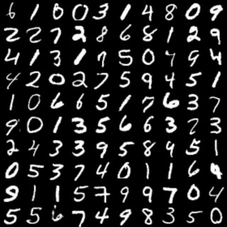
Then, we made models that would:

• Take an image of a digit and give you back the string value (ex: “2”) - post
• Take a string number value and give you back a digit image. - post

We will use both of the models to make a spec with a custom generator.

Note: For the sake of simplicity, some of the supporting code is left out. But if you want to see the whole code, it is on github)

With the help of the trained discriminator model, we can make a function that takes in an image and returns the number string value.

1
2
3
4
5
6
7
8

(defn discriminate [image]
  (-> (m/forward discriminator-model {:data [image]})
      (m/outputs)
      (ffirst)
      (ndarray/argmax-channel)
      (ndarray/->vec)
      (first)
      (int)))

Let’s test it out with a test-image:

1

(discriminate my-test-image) ;=> 6

Likewise, with the trained generator model, we can make a function that takes a string number and returns the corresponding image.

1
2
3
4

(defn generate [label]
  (-> (m/forward generator-model {:data [(ndarray/array [label] [batch-size])]})
      (m/outputs)
      (ffirst)))

Giving it a test drive as well:

1
2
3
4

(def generated-test-image (generate 3))
(viz/im-sav {:title "generated-image"
             :output-path "results/"
           :x (ndarray/reshape generated-test-image [batch-size 1 28 28])})

Great! Let’s go ahead and start writing specs. First let’s make a quick spec to describe a MNIST number - which is a single digit between 0 and 9.

1
2
3
4
5

(s/def ::mnist-number (s/and int? #(<= 0 % 9)))
(s/valid? ::mnist-number 3) ;=> true
(s/valid? ::mnist-number 11) ;=> false
(gen/sample (s/gen ::mnist-number))
;=> (0 1 0 3 5 3 7 5 0 1)

We now have both parts to validate and generate and can create a spec for it.

1
2
3
4
5
6

(s/def ::mnist-image
    (s/with-gen
      #(s/valid? ::mnist-number (discriminate %))
      #(gen/fmap (fn [n]
                   (do (ndarray/copy (generate n))))
                 (s/gen ::mnist-number))))

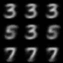
The ::mnist-number spec is used for the validation after the discriminate model is used. On the generator side, we use the generator for the ::mnist-number spec and feed that into the deep learning generator model to get sample images.

We have a test function that will help us test out this new spec, called test-model-spec. It will return a map with the following form:

1
2
3
4

{:spec name-of-the-spec
 :valid? whether or not the `s/valid?` called on the test value is true or not
 :sample-values This calls the discriminator model on the generated values
 }

It will also write an image of all the sample images to a file named sample-spec-name

Let’s try it on our test image:

1
2
3
4
5
6
7

(s/valid? ::mnist-image my-test-image) ;=> true


(test-model-spec ::mnist-image my-test-image)
;; {:spec "mnist-image"
;;  :valid? true
;;  :sample-values [0 0 0 1 3 1 0 2 7 3]}

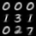
Pretty cool!

Let’s do some more specs. But first, our spec is going to be a bit repetitive, so we’ll make a quick macro to make things easier.

1
2
3
4
5
6
7

(defmacro def-model-spec [spec-key spec discriminate-fn generate-fn]
    `(s/def ~spec-key
       (s/with-gen
         #(s/valid? ~spec (~discriminate-fn %))
         #(gen/fmap (fn [n#]
                      (do (ndarray/copy (~generate-fn n#))))
                    (s/gen ~spec)))))

More Specs - More Fun

This time let’s define an even mnist image spec

1
2
3
4
5
6
7
8
9
10

 (def-model-spec ::even-mnist-image
    (s/and ::mnist-number even?)
    discriminate
    generate)

  (test-model-spec ::even-mnist-image my-test-image)

  ;; {:spec "even-mnist-image"
  ;;  :valid? true
  ;;  :sample-values [0 0 2 0 8 2 2 2 0 0]}

And Odds

1
2
3
4
5
6
7
8
9
10

  (def-model-spec ::odd-mnist-image
    (s/and ::mnist-number odd?)
    discriminate
    generate)

  (test-model-spec ::odd-mnist-image my-test-image)

  ;; {:spec "odd-mnist-image"
  ;;  :valid? false
  ;;  :sample-values [5 1 5 1 3 3 3 1 1 1]}

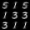
Finally, let’s do Odds that are over 2!

1
2
3
4
5
6
7
8
9
10

  (def-model-spec ::odd-over-2-mnist-image
    (s/and ::mnist-number odd? #(> % 2))
    discriminate
    generate)

  (test-model-spec ::odd-over-2-mnist-image my-test-image)

  ;; {:spec "odd-over-2-mnist-image"
  ;;  :valid? false
  ;;  :sample-values [3 3 3 5 3 5 7 7 7 3]}

Conclusion

We have shown some of the potential of integrating deep learning models with Clojure. clojure.spec is a powerful tool and it can be leveraged in new and interesting ways for both deep learning and AI more generally.

I hope that more people are intrigued to experiment and take a further look into what we can do in this area.

In this first post of this series, we took a look at a simple autoencoder. It took and image and transformed it back to an image. Then, we focused in on the disciminator portion of the model, where we took an image and transformed it to a label. Now, we focus in on the generator portion of the model do the inverse operation: we transform a label to an image. In recap:

• Autoencoder: image -> image
• Discriminator: image -> label
• Generator: label -> image (This is what we are doing now!)

Still Need Data of Course

Nothing changes here. We are still using the MNIST handwritten digit set and have an input and out to our model.

1
2
3
4
5
6
7
8
9
10
11
12
13
14
15
16
17
18
19
20

(def
  train-data
  (mx-io/mnist-iter {:image (str data-dir "train-images-idx3-ubyte")
                     :label (str data-dir "train-labels-idx1-ubyte")
                     :input-shape [784]
                     :flat true
                     :batch-size batch-size
                     :shuffle true}))

(def
  test-data (mx-io/mnist-iter
             {:image (str data-dir "t10k-images-idx3-ubyte")
              :label (str data-dir "t10k-labels-idx1-ubyte")
              :input-shape [784]
              :batch-size batch-size
              :flat true
              :shuffle true}))

(def input (sym/variable "input"))
(def output (sym/variable "input_"))

The Generator Model

The model does change to one hot encode the label for the number. Other than that, it’s pretty much the exact same second half of the autoencoder model.

1
2
3
4
5
6
7
8
9
10
11
12
13
14
15
16
17
18
19
20
21
22
23

(defn get-symbol []
  (as-> input data
    (sym/one-hot "onehot" {:indices data :depth 10})
    ;; decode
    (sym/fully-connected "decode1" {:data data :num-hidden 50})
    (sym/activation "sigmoid3" {:data data :act-type "sigmoid"})

    ;; decode
    (sym/fully-connected "decode2" {:data data :num-hidden 100})
    (sym/activation "sigmoid4" {:data data :act-type "sigmoid"})

    ;;output
    (sym/fully-connected "result" {:data data :num-hidden 784})
    (sym/activation "sigmoid5" {:data data :act-type "sigmoid"})

    (sym/linear-regression-output {:data data :label output})))

(def data-desc
  (first
   (mx-io/provide-data-desc train-data)))
(def label-desc
  (first
   (mx-io/provide-label-desc train-data)))

When binding the shapes to the model, we now need to specify that the input data shapes is the label instead of the image and the output of the model is going to be the image.

1
2
3
4
5
6
7
8
9
10

(def
  model
  ;;; change data shapes to label shapes
  (-> (m/module (get-symbol) {:data-names ["input"] :label-names ["input_"]})
      (m/bind {:data-shapes [(assoc label-desc :name "input")]
               :label-shapes [(assoc data-desc :name "input_")]})
      (m/init-params {:initializer  (initializer/uniform 1)})
      (m/init-optimizer {:optimizer (optimizer/adam {:learning-rage 0.001})})))

(def my-metric (eval-metric/mse))

Training

The training of the model is pretty straight forward. Just being mindful that we are using hte batch-label, (number label), as the input and and validating with the batch-data, (image).

1
2
3
4
5
6
7
8
9
10
11
12
13
14
15

(defn train [num-epochs]
  (doseq [epoch-num (range 0 num-epochs)]
    (println "starting epoch " epoch-num)
    (mx-io/do-batches
     train-data
     (fn [batch]
       ;;; change input to be the label
       (-> model
           (m/forward {:data (mx-io/batch-label batch)
                       :label (mx-io/batch-data batch)})
           (m/update-metric my-metric (mx-io/batch-data batch))
           (m/backward)
           (m/update))))
    (println "result for epoch " epoch-num " is "
             (eval-metric/get-and-reset my-metric))))

Results Before Training

1
2
3
4
5
6
7
8
9
10

(def my-test-batch (mx-io/next test-data))
  ;;; change to input labels
  (def test-labels (mx-io/batch-label my-test-batch))
  (def preds (m/predict-batch model {:data test-labels} ))
  (viz/im-sav {:title "before-training-preds"
               :output-path "results/"
               :x (ndarray/reshape (first preds) [100 1 28 28])})

  (->> test-labels first ndarray/->vec (take 10))
  ;=> (6.0 1.0 0.0 0.0 3.0 1.0 4.0 8.0 0.0 9.0)

Not very impressive… Let’s train

1
2
3
4
5
6
7
8
9

(train 3)

starting epoch  0
result for epoch  0  is
[mse 0.0723091]
starting epoch  1
result for epoch  1  is  [mse 0.053891845]
starting epoch  2
result for epoch  2  is  [mse 0.05337505]

Results After Training

1
2
3
4
5
6
7
8
9

 (def my-test-batch (mx-io/next test-data))
  (def test-labels (mx-io/batch-label my-test-batch))
  (def preds (m/predict-batch model {:data test-labels}))
  (viz/im-sav {:title "after-training-preds"
               :output-path "results/"
               :x (ndarray/reshape (first preds) [100 1 28 28])})
  (->> test-labels first ndarray/->vec (take 10))

  ;=>   (9.0 5.0 7.0 1.0 8.0 6.0 6.0 0.0 8.0 1.0)

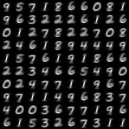
Cool! The first row is indeed

(9.0 5.0 7.0 1.0 8.0 6.0 6.0 0.0 8.0 1.0)

Save Your Model

Don’t forget to save the generator model off - we are going to use it next time.

1

(m/save-checkpoint model {:prefix "model/generator" :epoch 2})

Happy Deep Learning until next time …

In the last post, we took a look at a simple autoencoder. The autoencoder is a deep learning model that takes in an image and, (through an encoder and decoder), works to produce the same image. In short:

• Autoencoder: image -> image

For a discriminator, we are going to focus on only the first half on the autoencoder.

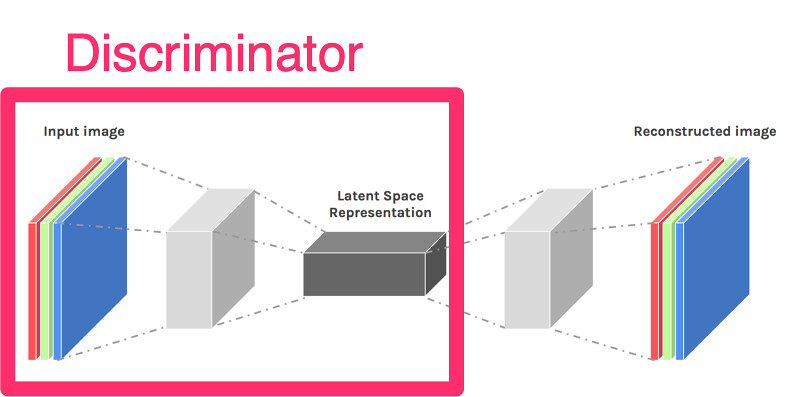
Why only half? We want a different transformation. We are going to want to take an image as input and then do some discrimination of the image and classify what type of image it is. In our case, the model is going to input an image of a handwritten digit and attempt to decide which number it is.

• Discriminator: image -> label

As always, with deep learning. To do anything, we need data.

MNIST Data

Nothing changes here from the autoencoder code. We are still using the MNIST dataset for handwritten digits.

1
2
3
4
5
6
7
8
9
10
11
12
13
14
15
16
17
18

;;; Load the MNIST datasets
(def train-data
  (mx-io/mnist-iter
   {:image (str data-dir "train-images-idx3-ubyte")
    :label (str data-dir "train-labels-idx1-ubyte")
    :input-shape [784]
    :flat true
    :batch-size batch-size
    :shuffle true}))

(def test-data
  (mx-io/mnist-iter
   {:image (str data-dir "t10k-images-idx3-ubyte")
    :label (str data-dir "t10k-labels-idx1-ubyte")
    :input-shape [784]
    :batch-size batch-size
    :flat true
    :shuffle true}))

The model will change since we want a different output.

The Model

We are still taking in the image as input, and using the same encoder layers from the autoencoder model. However, at the end, we use a fully connected layer that has 10 hidden nodes - one for each label of the digits 0-9. Then we use a softmax for the classification output.

1
2
3
4
5
6
7
8
9
10
11
12
13
14
15
16
17

(def input (sym/variable "input"))
(def output (sym/variable "input_"))

(defn get-symbol []
  (as-> input data
    ;; encode
    (sym/fully-connected "encode1" {:data data :num-hidden 100})
    (sym/activation "sigmoid1" {:data data :act-type "sigmoid"})

    ;; encode
    (sym/fully-connected "encode2" {:data data :num-hidden 50})
    (sym/activation "sigmoid2" {:data data :act-type "sigmoid"})

    ;;; this last bit changed from autoencoder
    ;;output
    (sym/fully-connected "result" {:data data :num-hidden 10})
    (sym/softmax-output {:data data :label output})))

In the autoencoder, we were never actually using the label, but we will certainly need to use it this time. It is reflected in the model’s bindings with the data and label shapes.

1
2
3
4
5

(def model (-> (m/module (get-symbol) {:data-names ["input"] :label-names ["input_"]})
               (m/bind {:data-shapes [(assoc data-desc :name "input")]
                        :label-shapes [(assoc label-desc :name "input_")]})
               (m/init-params {:initializer (initializer/uniform 1)})
               (m/init-optimizer {:optimizer (optimizer/adam {:learning-rage 0.001})})))

For the evaluation metric, we are also going to use an accuracy metric vs a mean squared error (mse) metric

1

(def my-metric (eval-metric/accuracy))

With these items in place, we are ready to train the model.

Training

The training from the autoencoder needs to changes to use the real label for the the forward pass and updating the metric.

1
2
3
4
5
6
7
8
9
10
11
12
13
14
15
16

(defn train [num-epochs]
  (doseq [epoch-num (range 0 num-epochs)]
    (println "starting epoch " epoch-num)
    (mx-io/do-batches
     train-data
     (fn [batch]
       ;;; here we make sure to use the label
       ;;; now for forward and update-metric
       (-> model
           (m/forward {:data (mx-io/batch-data batch)
                       :label (mx-io/batch-label batch)})
           (m/update-metric my-metric (mx-io/batch-label batch))
           (m/backward)
           (m/update))))
    (println {:epoch epoch-num
              :metric (eval-metric/get-and-reset my-metric)})))

Let’s Run Things

It’s always a good idea to take a look at things before you start training.

The first batch of the training data looks like:

1
2
3
4
5
6
7

  (def my-batch (mx-io/next train-data))
  (def images (mx-io/batch-data my-batch))
  (viz/im-sav {:title "originals"
               :output-path "results/"
               :x (-> images
                      first
                      (ndarray/reshape [100 1 28 28]))})

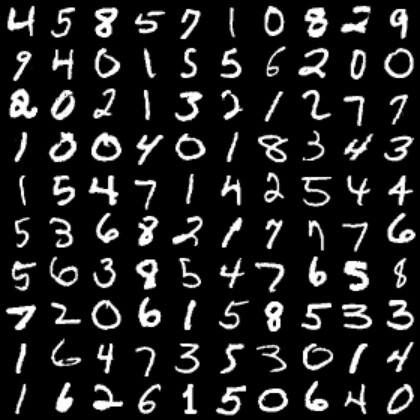
Before training, if we take the first batch from the test data and predict what the labels are:

1
2
3
4
5
6
7

  (def my-test-batch (mx-io/next test-data))
  (def test-images (mx-io/batch-data my-test-batch))
  (viz/im-sav {:title "test-images"
               :output-path "results/"
               :x (-> test-images
                      first
                      (ndarray/reshape [100 1 28 28]))})

1
2
3
4
5
6
7

  (def preds (m/predict-batch model {:data test-images} ))
  (->> preds
       first
       (ndarray/argmax-channel)
       (ndarray/->vec)
       (take 10))
 ;=> (1.0 8.0 8.0 8.0 8.0 8.0 2.0 8.0 8.0 1.0)

Yeah, not even close. The real first line of the images is 6 1 0 0 3 1 4 8 0 9

Let’s Train!

1
2
3
4
5
6
7
8

  (train 3)

;; starting epoch  0
;; {:epoch 0, :metric [accuracy 0.83295]}
;; starting epoch  1
;; {:epoch 1, :metric [accuracy 0.9371333]}
;; starting epoch  2
;; {:epoch 2, :metric [accuracy 0.9547667]}

After the training, let’s have another look at the predicted labels.

1
2
3
4
5
6
7

  (def preds (m/predict-batch model {:data test-images} ))
  (->> preds
       first
       (ndarray/argmax-channel)
       (ndarray/->vec)
       (take 10))
 ;=> (6.0 1.0 0.0 0.0 3.0 1.0 4.0 8.0 0.0 9.0)

• Predicted = (6.0 1.0 0.0 0.0 3.0 1.0 4.0 8.0 0.0 9.0)
• Actual = 6 1 0 0 3 1 4 8 0 9

Rock on!

Closing

In this post, we focused on the first half of the autoencoder and made a discriminator model that took in an image and gave us a label.

Don’t forget to save the trained model for later, we’ll be using it.

1
2

  (m/save-checkpoint model {:prefix "model/discriminator"
                            :epoch 2})

Until then, here is a picture of the cat in a basket to keep you going.

P.S. If you want to run all the code for yourself. It is here